9. 5. Solver Settings

9.5.1. Deformation solver (SOLMTD)

Solver

Sparse solver

Iteration Solver

Special Solver

Explicit Solver

Iteration methods (ITRMTH)

Direct

Newton-Raphson
9.5.2. Temperature solver (SOLMTT)

9.5.3. Induction Heating solver (SOLMTI)

9.5.4. Advanced

Convergence error limits (CVGERR)

Maximum number of iterations (ITRMXD, ITRMXT)

Bandwidth optimization (DEFBWD, TMPBWD)

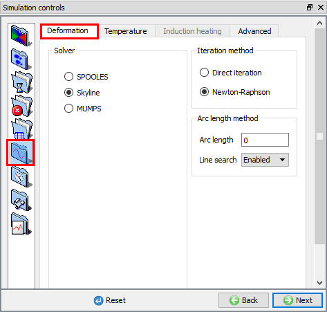
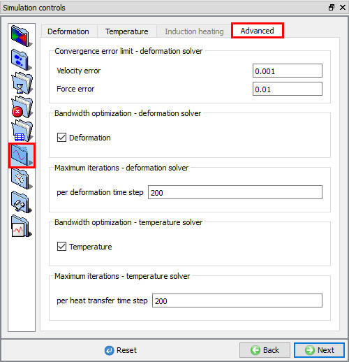
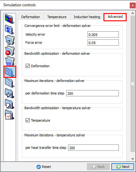
The Solver criteria specify criteria the FEM solver uses to find a solution at each step of the problem simulation. For most problems, the default values should be acceptable. It may be necessary to change the values if non-convergence occurs (See Fig. 9.5.1.)

(a)

(b)

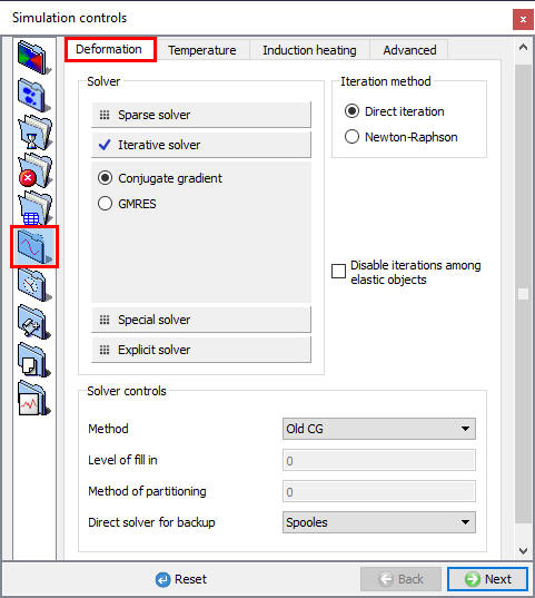
Solver settings for the Deformation solver; (a) For 2D (b) For 3D

Deformation solver (SOLMTD) [2D, 3D]

Solver

Sparse solver

The sparse (SOLMTD) solver takes advantage of the characteristics of the DEFORM matrix equations to solve the equations. It is efficient, especially for large problems.

SPOOLES and MUMPS [2D, 3D] :

The SPOOLES and MUMPS sparse matrix solvers are newer and more efficient, especially for larger problems. In the upcoming V12.0, the MUMPS solver with Newton-Raphson iteration method with be the new default for all simulations (plastic, elastoplastic, force-controlled, etc.).In 3D, It must be used on rotationally symmetric models with a brick mesh.

MUMPS [3D] :

Skyline [2D] :

The skyline solver is a very basic matrix inversion solution. It is the original solver that was used in DEFORM, and is maintained primarily for backward compatibility. It is robust, but not necessarily efficient.

Iteration Solver
Conjugate Gradient [3D]

The sparse (SOLMTD) solver is a direct solution that makes use of the sparseness of FEM formulation to improve solution speed. The conjugate-gradient solver tries to solve the FEM problem by iteratively approximating to the solution.

In V11.3, the default 3D solver for simulations with plastic objects is Conjugate gradient (CG) with direct iterations. Specifically, the ‘Old and New’ CG solver (Level of fill in = 4, Method of partitioning = 1) is the default with the MUMPS solver being the backup if needed for convergence. Elasto-plastic (EP) simulations cannot use the direct iteration method, so the recommendation for EP is the MUMPS solver with Newton-Raphson iterations.

GMRES [3D]

For certain problems, this solver offers tremendous advantages over the sparse solver.
The advantages of the iterative solver include:

Up to 5:1 improvements in overall solving time, particularly in very large problems
Ability to handle very large numbers of elements in reasonable time and with reasonable memory demands. (The largest problem to date is 380,000 tetrahedral elements, using 1GB of RAM on a 32bit PC). From 3Dv10.0, FEM engine has been further improved to take advantage of 64bit Linux environments thus being able to handle much larger model size.
Much smaller memory requirements for smaller problems - makes 3D practical on inexpensive computers or laptops.

Limitations:

In certain situations, convergence may be slower, or the simulation may not converge, when the sparse solver will converge. This is particularly a problem for simulations with large “rigid body motion” such as occurs when a part is settling into a die, undergoing light deformation, or bending.

When the conjugate-gradient solver cannot successfully converge toward the solution, DEFORM-3D will fall back to the sparse solver. From 3DV61, a new solver GMRES has been added to the available solvers, to take advantage of multiple CPU environments. The GMRES option can only be used in multi CPU mode.

When to use the iterative solver

**The solver is generally very good for problems with a lot of contact with the dies. If a workpiece is not well positioned in the dies, or if it will be sliding a bit before it starts deforming, you should start the simulation with the sparse solver. Once there is some substantial deformation in the workpiece, stop the simulation, load the final step into the pre-processor, change to “Conjugate Gradient” and “Direct”, and write the database. Fig. 9.5.2 gives the recommended Solver and Iteration methods for 3D model.
Keep an eye on the message file for the first few steps. The first step may be a bit slow converging. If the second step is still struggling to converge, or if the simulation stops, you may need to switch back to the sparse solver for a few more steps.
In general, simulations in which you might expect convergence problems using the Sparse solver are not well suited for Conjugate Gradient. Most problems, particularly thin parts or flash parts, will do well after the first 20-30 steps, if not sooner.

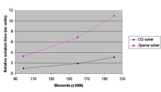
Plot of relative time versus elements for different solvers for Elastic Objects

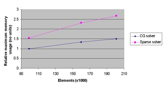
Plot of relative memory versus elements for different solvers for Elastic objects

Special Solver [3D]

The Special solver category contains several newly developed options intended to speed up the solving of very large 3D simulations (millions of elements).

Domain Decomposition (DD)

Domain decomposition (DD) splits the workpiece into several small sub-domains that can each be solved separately on different cores. It cannot be used with meshed tools or FEM-based volume compensation. Domain decomposition (DD) is based on MUMPS solver.

Domain decomposition method can be used only for Rigid Plastic object types with tet mesh.

Domain decomposition may be faster for very large problems.

Dual Mesh (DM)

Dual mesh (DM) simultaneously uses both a fine and coarse mesh on the workpiece, where the solution on the coarse mesh is used as the initial guess for the fine mesh. This can substantially improve the solving speed of the CG solver.

“Dual mesh size factor” N will control the coarse mesh size., the number of elements for coarse mesh will be 1/N of original workpiece.

8 is default value in Gui-Pre. 5~10 can be possible.

DD+DM

It decomposes the model to spread the solution across processors, Runtime can be improved on large elasto-plastic models. DD+DM is still maturing, but feel free to try it to determine if your application benefits from its techniques.
It cannot be used with meshed tools or FEM-based volume compensation.
DD+DM is its own unique solver, it is based on elements of the DD and DM solvers.

Partial domain Solver : “Partial domain solver ” is available under Special solvers and is currently available only for “Lagrangian incremental” and “ALE spinning” simulation type. This solver simulates localized deformation within the specified active domain. Under Partial domain, user have options to use Quick Evaluation. Quick evaluation can allow moving rotation center along the selected axis. User can define the active domain for the objects to be considered for calculation from the table under Solver controls. Inactive domain over the workpiece can be defined from the Property page of the Workpiece.
- Quick evaluation Solver : Quick evaluation solver solves one step (per revolution) model for incremental rotary forming and is currently available only for ALE Spinning. Quick Evaluation Method with partial domain solver can improve the computational efficiency and is good for the parametric study for initial check of the processing design.
- Quick evaluation with moving rotation center : We can select this option to update the moving rotation center of the objects in the selected direction from Direction pull down list.
- Active domain total angle : Using this option we can define the total angle of the active domain within which the calculations are performed.
- Rotation axis : This option is used to define the rotation axis of the object. For the selected rotation axis, we can define Inactive domain from the Property page - Partial domain tab of the Workpiece.
- Preview : Using this preview button, we can observe the active domain for the partial domain calculation zone on the workpiece. Active domain will be highlighted in White color in display region as shown in Fig. 9.5.4.
- Add : Using this button, we can add objects to the list for which active domain will be defined, if not added by default. Currently, the objects which are having translation (Speed, Path) movement data will be added to the table by default.
- Delete : Using this button, we can delete the added objects from the list.
- Boundary constraints :
  1. Methods : Under methods pulldown list, we have Bar stiffness or Penalty spring methods that can be applied to the Partial Domain.
  2. Scalingfactor : using this option, we can define the scaling factor value for the boundary constraints.

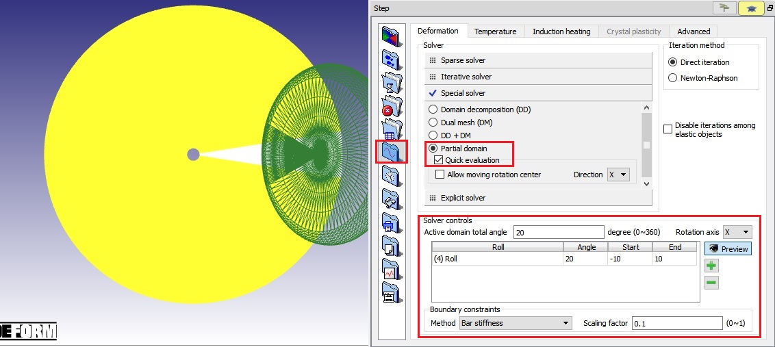
Partial domain solver options

Explicit Solver [3D]:
Explicit:

An explicit solver is now available for 3D simulations. An explicit solver does not require any iterations and the nodal velocities are solved directly. Explicit solvers are typically used to simulate processes which have a very short time duration (such as automobile crashes). The time step in an explicit analysis must be very small - less than the time it takes a sound wave to travel across an element. Implicit simulations, on the other hand, do not have an inherent time step size limit, so implicit time steps are generally several orders of magnitude larger than explicit time steps. If the process being modeled is very short, or the time steps are required to be very small, the explicit solver might be a good fit. Contact DEFORM Technical Support if you would like to try the explicit solver.

Solver recommendations:

Now that the solvers for 2D and 3D have been described, it would be helpful to have a table detailing the recommended solvers for various model setups.

2D

As the table shows, the MUMPS solver is recommended in all situations. For small problem sizes, all the solvers will have essentially the same speed. As the problem size increases, the MUMPS solver becomes the fastest option.

3D

Solver selection in 3D is less straightforward than 2D. Most 3D DEFORM simulations have one Plastic workpiece and velocity-controlled Rigid tools. These simulations should use the CG solver. Elasto-plastic simulations should use the MUMPS solver. The recommended solver for all other scenarios can be found in the above table.

Iteration methods (ITRMTH) [2D, 3D]

An iteration method (ITRMTH) is the manner in which the simulation solution is updated (or iterated upon) to try to approach the converged step solution.

Direct

The direct method is more likely to converge than Newton-Raphson, but will generally require more iterations to do so. In the case of Porous materials, the direct method is the only method currently available.

Newton-Raphson

The Newton-Raphson method is recommended for most problems because it generally converges in fewer iterations than the other available methods. However, solutions are more likely to fail to converge with this method than with other methods.

Arc -Length method
Disable iterations among elastic objects

Temperature solver (SOLMTT) [2D, 3D]

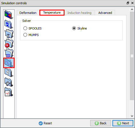
(a)

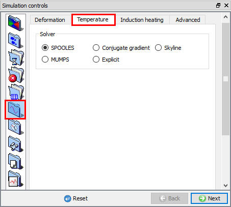
(b)

Temperature iteration settings; (a) For 2D (b) For 3D

SPOOLS[2D, 3D]
Skyline[2D, 3D]

While the Sparse solver is efficient for large size models, the skyline solver uses the skyline storage method in conjunction with Gaussian elimination to store temperature matrix data. This method is recommended for most problems.

MUMPS [2D, 3D]
Conjugate Gradient [3D]

Compared to other type of solvers, Conjugate-Gradient solver requires much less memory and results in faster solutions times for large size models.

Explicit [3D]

Induction Heating solver (SOLMTI) [3D]

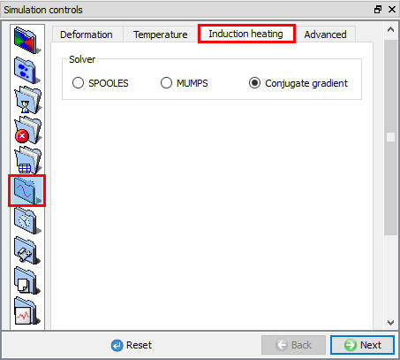
Induction Heating solver settings

Advanced

(a)

(b)

Advanced solver settings; (a) For 2D (b) For 3D

Convergence error limits (CVGERR) [2D, 3D]

Deformation iteration is assumed to have converged when the velocity and force error limits (CVGERR) have been satisfied. This means that the change in both the nodal velocity norm and the nodal force norm is below the value specified as shown in Fig 9.5.7. The error norm values for each iteration step are displayed in the message file. If the message file shows that the force or velocity error norms are getting small, but not dropping below the error limits, the simulation may be continued by increasing the appropriate error limit to the smallest value in the message file. This will decrease the solution accuracy, so the simulation should be allowed to run a few steps, then the values should be reduced again. When doing this, extreme care should be exercised.

For die stress or press load calculations where extremely accurate force or load values are required, the load accuracy may be improved by decreasing the force error limit. This will increase simulation time, but give more accurate results.

Note:
It should be noted that the accuracy of the flow stress data will have great impact on the accuracy of die stress and press load predictions.

Maximum number of iterations (ITRMXD, ITRMXT) [2D, 3D]

When Newton-Raphson iteration is being used, the specified number of iterations (ITRMXD and ITRMXT) will be performed for each iteration segment until the solution has converged. At most, 30 iterations will be performed during a Newton-Raphson segment. If the solution does not converge in the specified number of iterations, and with automatic step size reduction that follows, the simulation will terminate and a message will be written to the DEFORM message file.
If direct iteration is specified as the iteration method, the specified number of iterations will be performed. If the solution has not converged, another series of iterations will be performed. If the solution has still not converged, the simulation will terminate, and a message will be written to the DEFORM message file.

Bandwidth optimization (DEFBWD, TMPBWD)[2D, 3D]

Bandwidth optimization (DEFBWD and TMPBWD) improves solution time by optimizing the structure of the matrix equation being solved. It should be used for almost all problems.