Lab2 Square Ring
2.1. Introduction
2.2. Creating a New Problem
2.3. Adding Operation
2.4. Adding Objects
2.5. Workpiece
2.6. Top Die
2.7. Inter-Object relationships
2.8. Step Controls
2.9. Database Generation
2.10. Running Simulation
2.11. Post Processing
Introduction
Symmetry should be taken advantage of whenever possible in simulations. Doing so saves computational time and can increase solution accuracy. Furthermore, the smallest possible section that adequately describes the problem should be modeled.
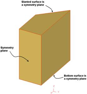
In this lab, we will simulate the upsetting of a square ring. The square ring has quite a bit of symmetry that can be taken advantage of. This lab will show you that the deformation of the entire ring can be determined by only modeling 1/16 of its full geometry.
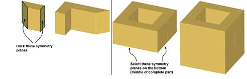
Sectioning of Square ring modeled for analysis
Creating a New Problem
On a Windows machine , go to the ![]() button select DEFORM-v1x.xxx (.xxx indicates version number E.g. v14.0.2) and select DEFORM GUI Main vxx.xx from the menu. The DEFORM GUI Main window will appear as shown below Fig. 3DL2.2.
button select DEFORM-v1x.xxx (.xxx indicates version number E.g. v14.0.2) and select DEFORM GUI Main vxx.xx from the menu. The DEFORM GUI Main window will appear as shown below Fig. 3DL2.2.
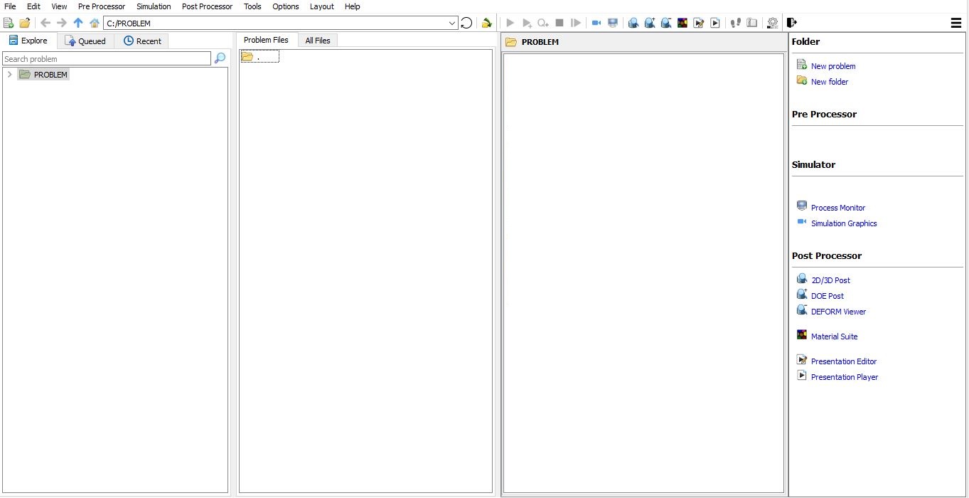
DEFORM GUI main window
Create a new problem either by selecting File ![]() New Problem or by clicking the New Problem
New Problem or by clicking the New Problem ![]() icon. The Problem Setup window will appear as shown in Fig. 3DL2.3. Select “Integrated Manufacturing Process “ radio button and unit system as “English “ radio button in unit field. Define Problem Name as “ **Square_Ring** “ and make sure the “Show option dialog ” check box is turned on (if we do not turn on the “Show option dialog” check box, then we will not get the New Project dialog). Then click on
icon. The Problem Setup window will appear as shown in Fig. 3DL2.3. Select “Integrated Manufacturing Process “ radio button and unit system as “English “ radio button in unit field. Define Problem Name as “ **Square_Ring** “ and make sure the “Show option dialog ” check box is turned on (if we do not turn on the “Show option dialog” check box, then we will not get the New Project dialog). Then click on ![]() button to open a new problem using the Deform Integrated Manufacturing Process.
button to open a new problem using the Deform Integrated Manufacturing Process.
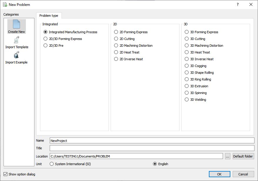
Problem type selection window
Multiple operation wizard will open with the New Project dialog (see Fig. 3DL2.4.), at this point user will be prompted to specify a project name (system will create a separate folder with this project name) and title for this session. In this session we use ‘Square_Ring ’ as the project name.
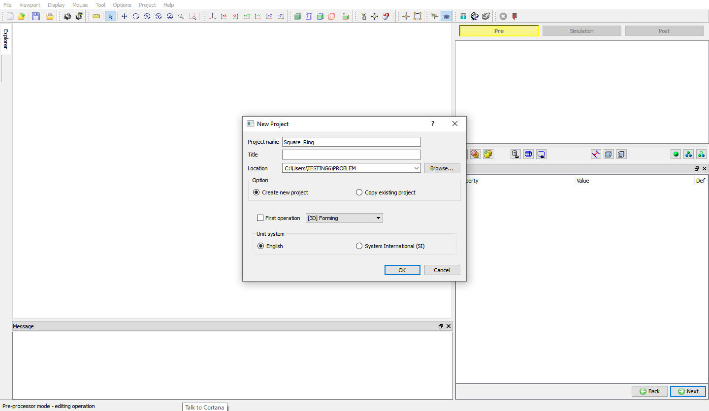
New Project selection window
User can also change the Unit system (File menu selected unit system will be selected by default) and add operation by selecting from First operation pull down list and checkbox (see Fig. 3DL2.5.). Using copy Existing project option we can import previous saved projects as new project. Click on ![]() to continue to open the operation.
to continue to open the operation.
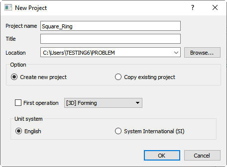
Assigning problem name
To simulate the forging of this square ring, only a workpiece and a top die are required - the bottom die is not needed due to symmetry.
Adding Operation
Add 3D Forming operation from the Explorer Operations list. Add the operation by clicking on ![]() button available next to 3D Forming or user can also add by drag and drop into the Operation editor. (See Fig. 3DL2.6.)
button available next to 3D Forming or user can also add by drag and drop into the Operation editor. (See Fig. 3DL2.6.)
Operation Explorer
In this operation we are setting up simple Isothermal operation so, in Simulation control page Sim Mode tab, turnoff the Heattransfermode check box. Click on ![]() .
.
In Material list window, load the ‘AISI-1045, COLD ‘ material from DEFORM Material library, Steel category using ![]() (Load material data from library) option. This can be done as shown in below Fig. 3DL2.7. by clicking
(Load material data from library) option. This can be done as shown in below Fig. 3DL2.7. by clicking ![]() button. Click on
button. Click on ![]() .
.
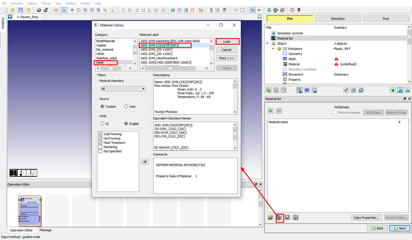
Material library window
Adding Objects
If there aren’t already two objects, add the two objects by clicking the insert object ![]() button. The two objects will be named as Workpiece and Top Die. If there are three objects, delete the Bottom Die by selecting it and clicking the Delete selected
button. The two objects will be named as Workpiece and Top Die. If there are three objects, delete the Bottom Die by selecting it and clicking the Delete selected ![]() object button (see Fig. 3DL2.8.), then click on
object button (see Fig. 3DL2.8.), then click on ![]() .
.
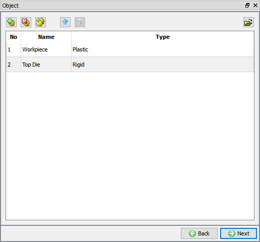
Object Window
Workpiece
In Workpiece window, change the Object name to Billet and select Object type as Plastic and temperature as68°F as shown in Fig. 3DL2.9. Click on ![]() .
.
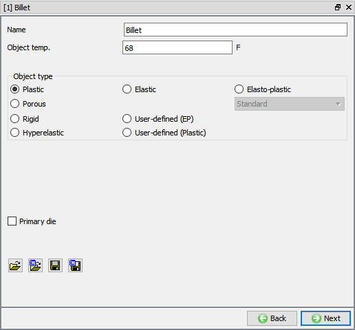
Billet object Window
Loading Billet Geometry
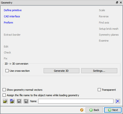
In Geometry window, load SquareRing_Billet.STL geometry file from library using (Load geometry from library) option or can also be imported using ![]() (Load geometry from a file ) option as shown in Fig. 3DL2.10. The geometry is located in DEFORM installation folder \3d\LABS directory. Check the geometry using the
(Load geometry from a file ) option as shown in Fig. 3DL2.10. The geometry is located in DEFORM installation folder \3d\LABS directory. Check the geometry using the ![]() and
and ![]() options.
options.
Billet Geometry window
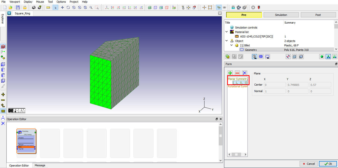
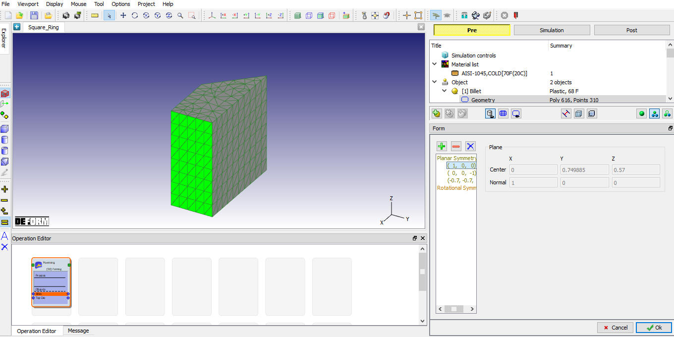
Symmetry is being taken advantage of in this simulation and only 1/16 of the square ring is being modeled. Using Planar symmetry option define the symmetry planes to enforce the correct deformation (see Fig. 3DL2.11.). Click on ![]() , under Planar Symmetry select the symmetry plane that is normal to the X-axis (as shown below Fig. 3DL2.12.). The selected plane polygon face on the Plane will get highlighted and the Plane Information will be listed in the Plane area.
, under Planar Symmetry select the symmetry plane that is normal to the X-axis (as shown below Fig. 3DL2.12.). The selected plane polygon face on the Plane will get highlighted and the Plane Information will be listed in the Plane area.
Symmetry Plane
Click the ![]() button to add symmetry boundary conditions. This symmetry plane will now be listed in the Planar symmetry list as (1, 0, 0) which is the normal to the X plane. (See Fig. 3DL2.12.)
button to add symmetry boundary conditions. This symmetry plane will now be listed in the Planar symmetry list as (1, 0, 0) which is the normal to the X plane. (See Fig. 3DL2.12.)
Assigned Planar symmetry on X Plane
Repeat the above procedure to add the Planar symmetry for the other two symmetry planes. First select the symmetry plane, so that the selected plane get highlighted and then use the ![]() button to add them. When all three symmetry planes have been added, the planar symmetry area should look like as shown in Fig. 3DL2.13. then click on
button to add them. When all three symmetry planes have been added, the planar symmetry area should look like as shown in Fig. 3DL2.13. then click on ![]() in Planar symmetry page and click on
in Planar symmetry page and click on ![]() to generate mesh.
to generate mesh.
Assigned Planar Symmetry data for geometry
Meshing the Billet
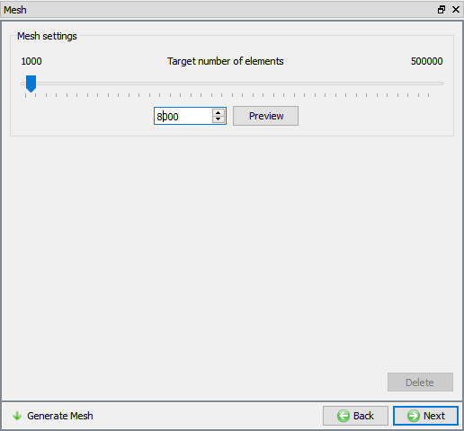
In Mesh window, change theTarget number of elements to 8000 and click on ![]() button. The surface mesh that is created looks good. So click the
button. The surface mesh that is created looks good. So click the ![]() button to finish the meshing process. (See Fig. 3DL2.14.) When meshing is completed, the object should have around 5000 elements. When you are asked “Do you want to assign default boundary conditions?” click
button to finish the meshing process. (See Fig. 3DL2.14.) When meshing is completed, the object should have around 5000 elements. When you are asked “Do you want to assign default boundary conditions?” click ![]() . Click on
. Click on ![]() to material page.
to material page.
Billet Mesh window
Assigning Material to the Billet
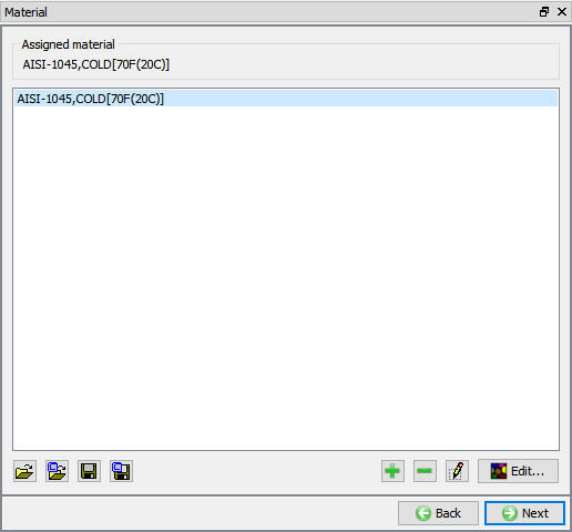
To assign material for workpiece select the material AISI-1045 COLD from material window. This can be done as shown in below Fig. 3DL2.15. Click ![]() to Boundary condition page .
to Boundary condition page .
Billet Material window
Setting symmetry boundary conditions
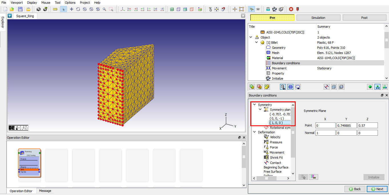
In Boundary condition page observe the assigned Symmetry plane data, the Boundary Condition area should look like as shown in Fig. 3DL2.16.
Since it is isothermal setup, delete the default assigned Heat exchange with environment BCC. Click ![]() until top die object window.
until top die object window.
Symmetry boundary conditions
Top die
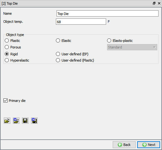
In Top die object window, keep the object type as rigid and temperature as 68°F, also make sure the primary die check box is checked and click ![]() . (See Fig. 3DL2.17.)
. (See Fig. 3DL2.17.)
Top die object window
Loading Top die Geometry
In Geometry window, load SquareRing_TopDie.STL geometry file from library using ![]() (Load geometry from library) option. The geometry is located in DEFORM installation folder \3d\LABS directory. Check the geometry using the
(Load geometry from library) option. The geometry is located in DEFORM installation folder \3d\LABS directory. Check the geometry using the ![]() and
and ![]() options, then click
options, then click ![]() until the Movement window. Since this is an isothermal problem no mesh nor related data need to be specified.
until the Movement window. Since this is an isothermal problem no mesh nor related data need to be specified.
Assigning Movement to Top die
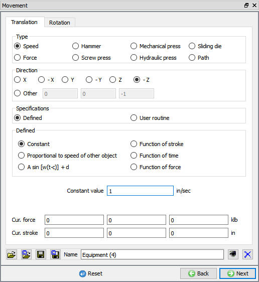
Define a speed of 1 in/sec in -Z direction. Click ![]() until the Contact window appears as both the Billet and top die are in right position. (See Fig. 3DL2.18.)
until the Contact window appears as both the Billet and top die are in right position. (See Fig. 3DL2.18.)
Top Die Movement window
Inter-Object relationships
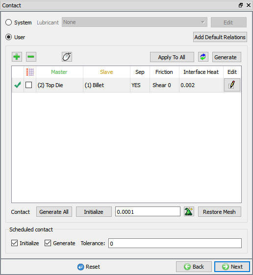
Select user type radio button and click on ![]() button. It will add the relationship between the Billet and the Top Die as shown in Fig. 3DL2.19.
button. It will add the relationship between the Billet and the Top Die as shown in Fig. 3DL2.19.
Inter-Object window
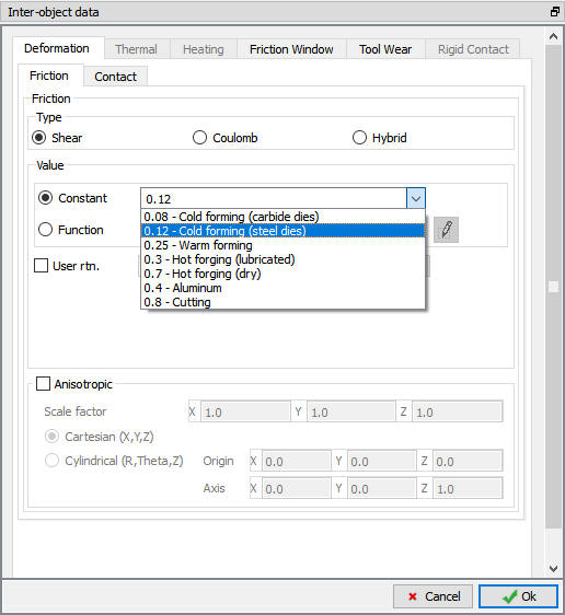
Define the friction for the relationship by clicking the ![]() button. Use the pull-down menu to select the friction suitable for Cold forming (steel dies). (See Fig. 3DL2.20.)
button. Use the pull-down menu to select the friction suitable for Cold forming (steel dies). (See Fig. 3DL2.20.)
Inter-Object data definition window
Click ![]() to go back to Inter-Object window, use
to go back to Inter-Object window, use ![]() icon to determine a suitable contact tolerance (a value of about 0.00192” will be calculated) and then click
icon to determine a suitable contact tolerance (a value of about 0.00192” will be calculated) and then click ![]() button to generate contact. If you rotate the objects around in graphics window, you will see that contact was generated between the two objects. Click
button to generate contact. If you rotate the objects around in graphics window, you will see that contact was generated between the two objects. Click ![]() until Step window as no Stopping controls aren’t necessary.
until Step window as no Stopping controls aren’t necessary.
Step Controls
In Step controls window change the preprocessor setup mode to Expert by using the ![]() (Switch to expert mode) icon from the tool bar. Expert mode will provide more options for detailed settings. (See Fig. 3DL2.21.)
(Switch to expert mode) icon from the tool bar. Expert mode will provide more options for detailed settings. (See Fig. 3DL2.21.)
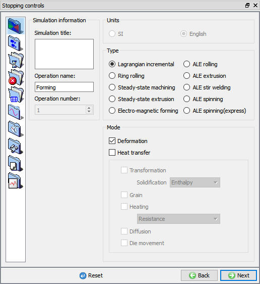
Step controls Main tab in expert mode
Select the steps tab (![]() ), set the Number of Simulation Steps to 30 and StepIncrementtoSave to 2. Set the TopDie as PrimaryDie. (See Fig. 3DL2.22.)
), set the Number of Simulation Steps to 30 and StepIncrementtoSave to 2. Set the TopDie as PrimaryDie. (See Fig. 3DL2.22.)
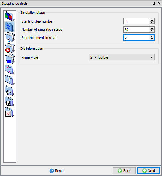
Step controls Simulation Steps tab in expert mode
To determine an appropriate step size, select the ![]() icon and measure the edge length of a few of the smaller elements in the Billet. An average length of a short edge is around 0.06”. Use a Constant Die Displacement per step of 0.02 in/step, which is 1/3 of this small edge length in step increment tab (
icon and measure the edge length of a few of the smaller elements in the Billet. An average length of a short edge is around 0.06”. Use a Constant Die Displacement per step of 0.02 in/step, which is 1/3 of this small edge length in step increment tab (![]() ) for step size as die displacement. (See Fig. 3DL2.23.)
) for step size as die displacement. (See Fig. 3DL2.23.)
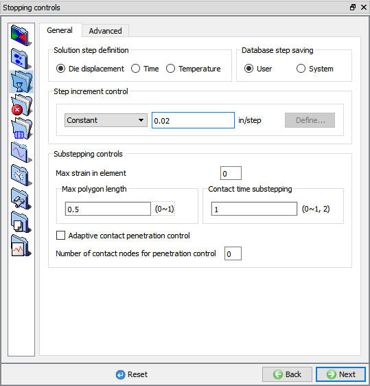
Simulation controls Step increment tab in expert mode
Click ![]() and save a keyword file for the problem by selecting the File menu Export option.
and save a keyword file for the problem by selecting the File menu Export option.
Database Generation
Click on ![]() action label to check the problem. The only warning should deal with Volume Compensation appear in the console window - ignore this for this lab. Generate a database by clicking
action label to check the problem. The only warning should deal with Volume Compensation appear in the console window - ignore this for this lab. Generate a database by clicking ![]() action label.
action label.
Running Simulation
Once the database has been generated, switch to the Simulation mode by clicking on ![]() button above the operation tree.
button above the operation tree.
Click on the ![]() action label to open the Run Options dialog Use the default Continue Run option to select “Continue from the last step ” option and then select the Simulation mode as Interactive and click on
action label to open the Run Options dialog Use the default Continue Run option to select “Continue from the last step ” option and then select the Simulation mode as Interactive and click on ![]() button to run the simulation.
button to run the simulation.
Monitor the progress of the simulation by looking at the Simulation graphics window and Simulation Message and Simulation Log tabs, making sure that the ![]() option is checked (See). Simulation graphics tool bar options can be used to plot basic state variables and contact for objects while simulating the problem.
option is checked (See). Simulation graphics tool bar options can be used to plot basic state variables and contact for objects while simulating the problem.
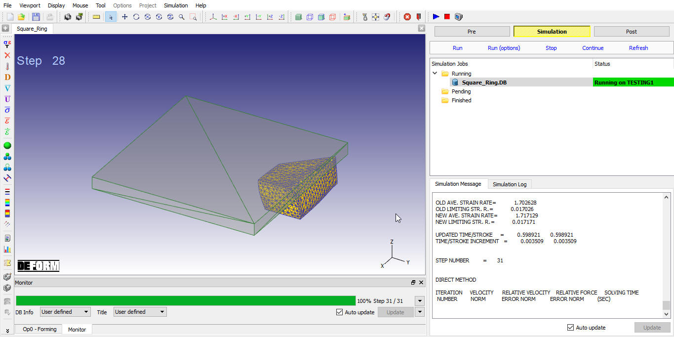
MO Simulation Mode
Post Processing
When the simulation is complete, review the results by switching to Post mode using the button above the Simulation tool bar. (See Fig. 3DL2.25.)
In reality this part is a full square ring, so it would be useful to be able to view the entire part in the Post-processor. To create the entire object, the small 1/16 section has to be mirrored about the symmetry planes. Clicking the ![]() icon open the 3D Mirroring window. (See Fig. 3DL2.26.)
icon open the 3D Mirroring window. (See Fig. 3DL2.26.)
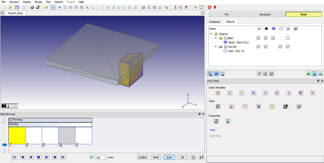
MO Post Mode
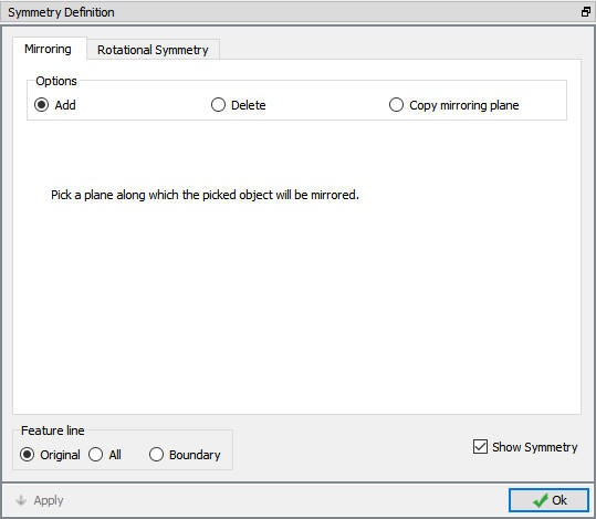
3D Mirroring window
Use the mouse to click on the symmetry planes on the Billet. Each time this is done a mirror image of the billet will be displayed. Repeat the process until the entire billet is shown. This procedure is illustrated below. (See Fig. 3DL2.27.)

Symmetry definition
Once the complete part is displayed in the Graphics window, close the Symmetry definition window by clicking OK. Play through the steps to observe how the square ring deforms as it is compressed. Experiment with viewing the different state variables such as effective strain. (See Fig. 3DL2.28.)
Strain effective result
When finished viewing the results of the simulation, use the ![]() icon to return to the GUI Main window.
icon to return to the GUI Main window.
Related Topics: