3D Inverse Heat Lab1

Problem Summary

This lab will demonstrate how to use the Inverse Heat Transfer Wizard to determine heat transfer coefficients between workpiece and media during a heat transfer process. Temperature measurement data is needed. Heat transfer coefficients can be function of temperature or time. Multiple zones of heat-transfer coefficients are assigned to the workpiece

1.1. Starting a new problem

1.2. Mode selection page

1.3. Setting Process Conditions

1.4. Defining Material

1.5. Defining Workpiece Object

1.6. Import geometry

1.7. Generate mesh

1.8. Assigning Material

1.9. BCC Definition

1.10. Temperature Measurement Points

1.11. Defining Time Zones

1.12. Defining Heat Transfer Zones

1.13. Defining Step controls

1.14. Optimization control

1.15. Database Generation

1.16. Optimization

1.17. Optimization results

Starting a new problem

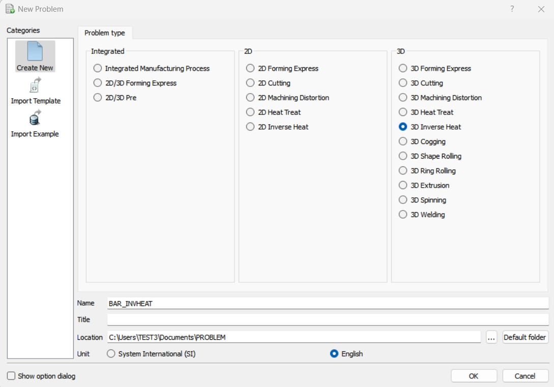
Start a new Inverse Heat Transfer Wizard problem with problem ID BAR_INVHEAT. You can do so by clicking the button and choose “3D InverseHeat ” Problem type along with “English ” for “Unit System” (see Fig. 3DINVL1.1.). You can select the directory for the project under Location filed and then click to open Inverse Heat wizard.

Problem Setup window

Mode selection page

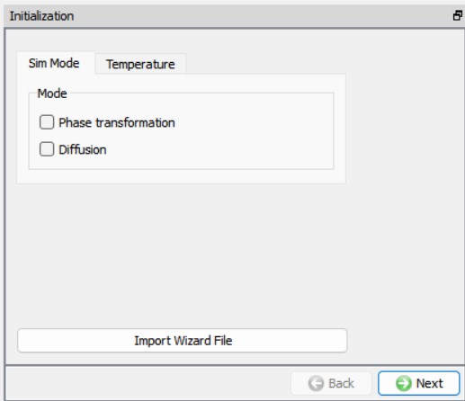
As the 3D Inverse Heat wizard opens, you should see a window as shown in Fig. 3DINVL1.2. If user is interested in calculating transformations or atom content due to diffusion then user can turn on respective check boxes under “Sim Mode” tab. In this lab we will not turn on any check box as we will be calculating only heat transfer co-efficients. Click .

Initialization Window

Setting Process Conditions

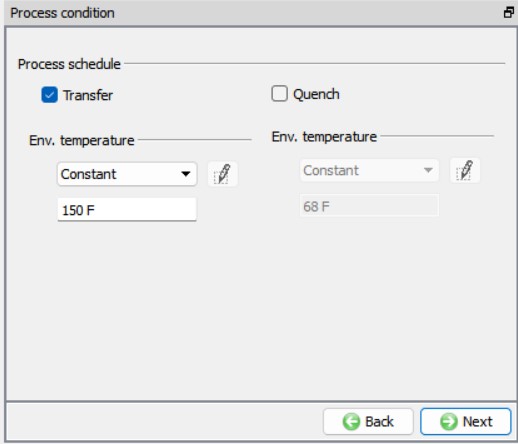
User can set the environment conditions in this page. If the process involves Quenching and heat transfer, then respective check boxes can be turned on to define the environment conditions. Our process involves only heat transfer and the environmental temperature is constant. Hence, turn off “Quench”, turn on “Transfer ” and define environment temperature as 150F(See Fig. 3DINVL1.3.). Click .

Setting up Process conditions

Defining Material

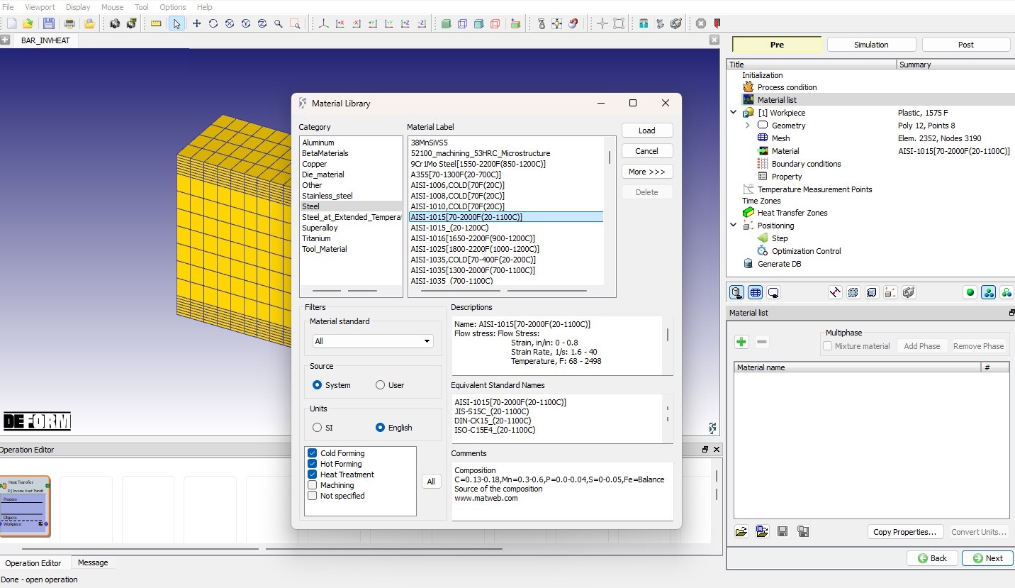
In page “Material**list** ”, choose and in the material library, choose “Steel “ category and load “AISI-1015[70-2000F(20-1100C)] “ as shown in Fig. 3DINVL1.4. Click on until “Workpiece” page.

Loading Material data from library

Defining Workpiece Object

In workpiece page, define “Object Temp.” as 1575F as shown in Fig. 3DINVL1.5. Make sure the object type is Plastic and Primary Die check box is checked. Click .

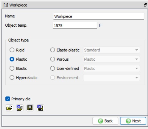
Workpiece Object Definition

Import geometry

In “Geometry” page, click on icon and import geometry file “BAR_INVHEAT.STL ” from ‘/3d/LABS’ directory as shown in Fig. 3DINVL1.6. Click Setup brick mesh to open the dialog. Select Extrude radio button and pick Workpiece surface on the +Z direction as Start surface and the surface in -Z direction as End surface, see Fig. 3DINVL1.7. Click the button to close the “Setup brick mesh” dialog, then click on to open the ‘Symmetry’ dialog. In Symmetry dialog, select Planar surface and then pick Workpiece surfaces in +X and -Y direction as planar symmetry faces. To mark each plane, select the face and then click , see Fig. 3DINVL1.8. Click the button to close the “Symmetry” dialog, then click to generate mesh.

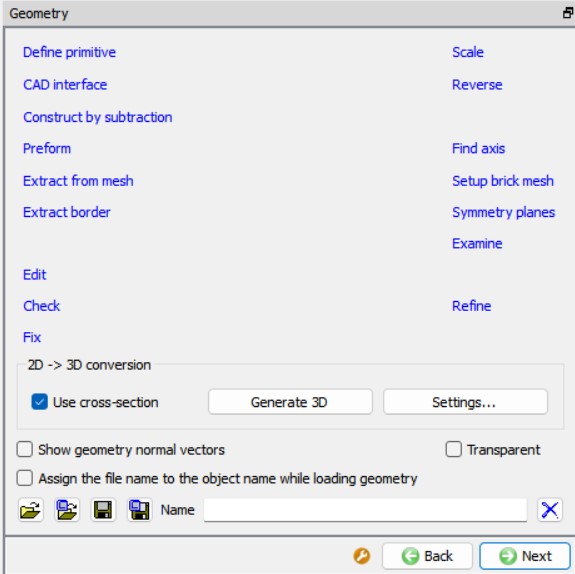
Geometry page

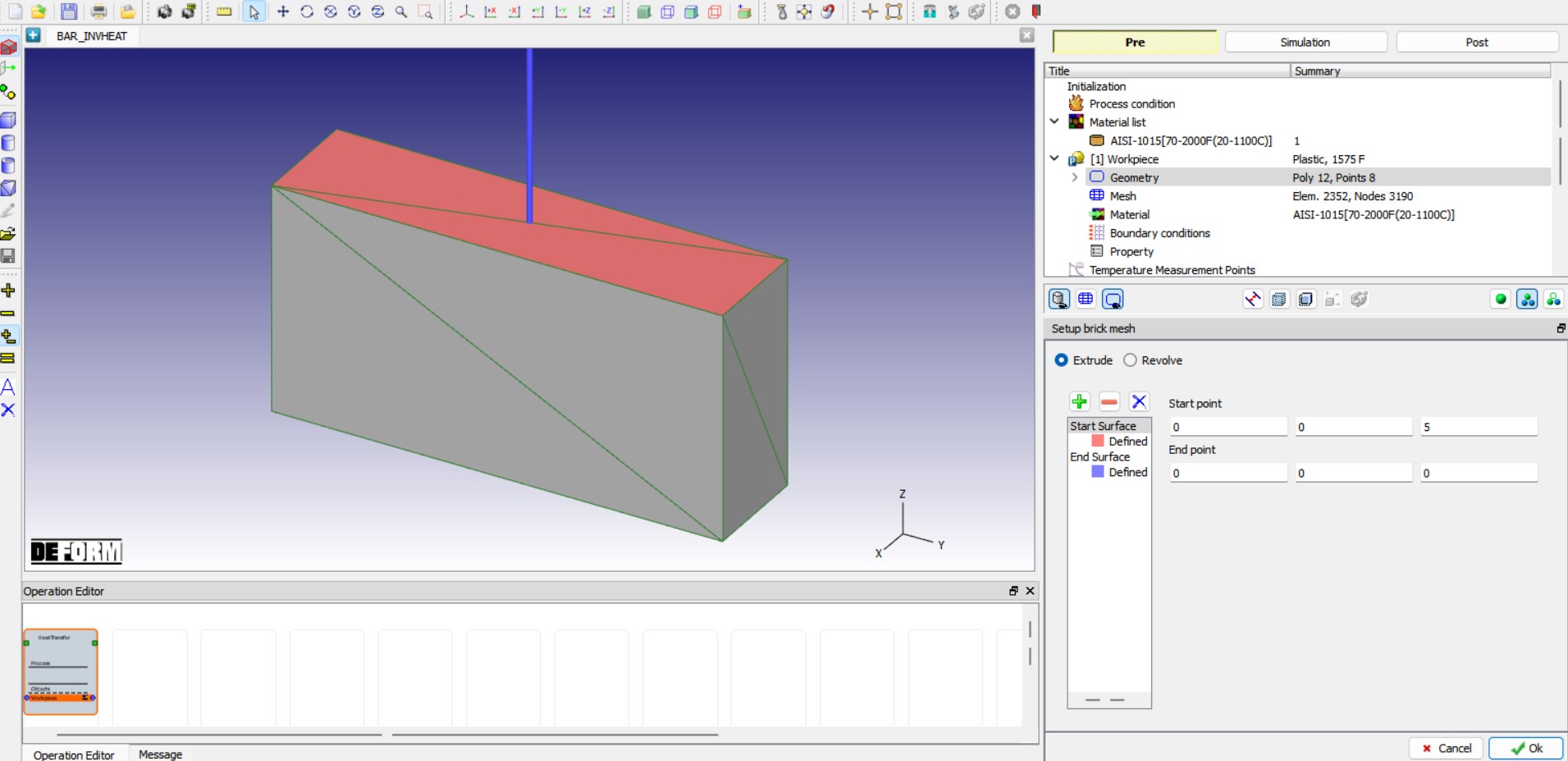
Setup Brick mesh page

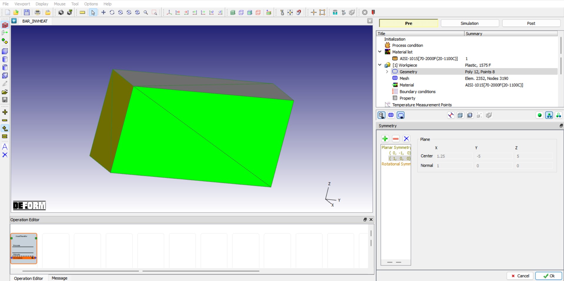
Assigned symmetry plane data

Generate mesh

While user is in “Mesh” page, expert mode can be used to access the advanced mesh options. Click on n icon in tool bar to change to expert mode and select Brickmesh radio button. From Brick mesh options, select Finer mesh area radio button and click on button three times to add three finer mesh areas (0 - 0.59, 0.59 - 4.41, 4.41 - 5) and define no of layers as ‘7’ for all three finer mesh areas, see Fig. 3DINVL1.9.
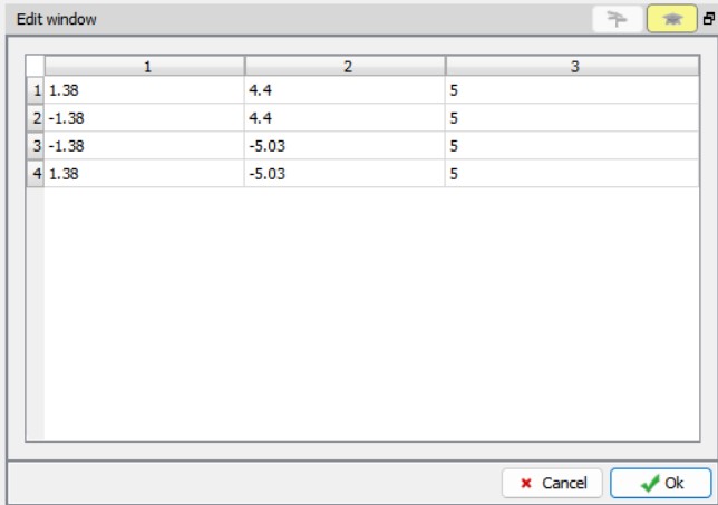
Select 2D cross section tab, define target number of elements as ‘110 ’, Thickness elements as ‘4 ’, sizeratio as ‘10 ’ and turn on Mapped mesh checkbox. Click on weighting factors tab and define mesh windows as ‘1 ’ . Click on mesh windows tab and add a mesh window over the 2D mesh, select window 1 and define values by clicking on button as shown in Fig. 3DINVL1.9. Define Relative element size as ‘100 ’ and select Workpiece as follow object. Click on button to generate brick mesh. Click on to assign Material.

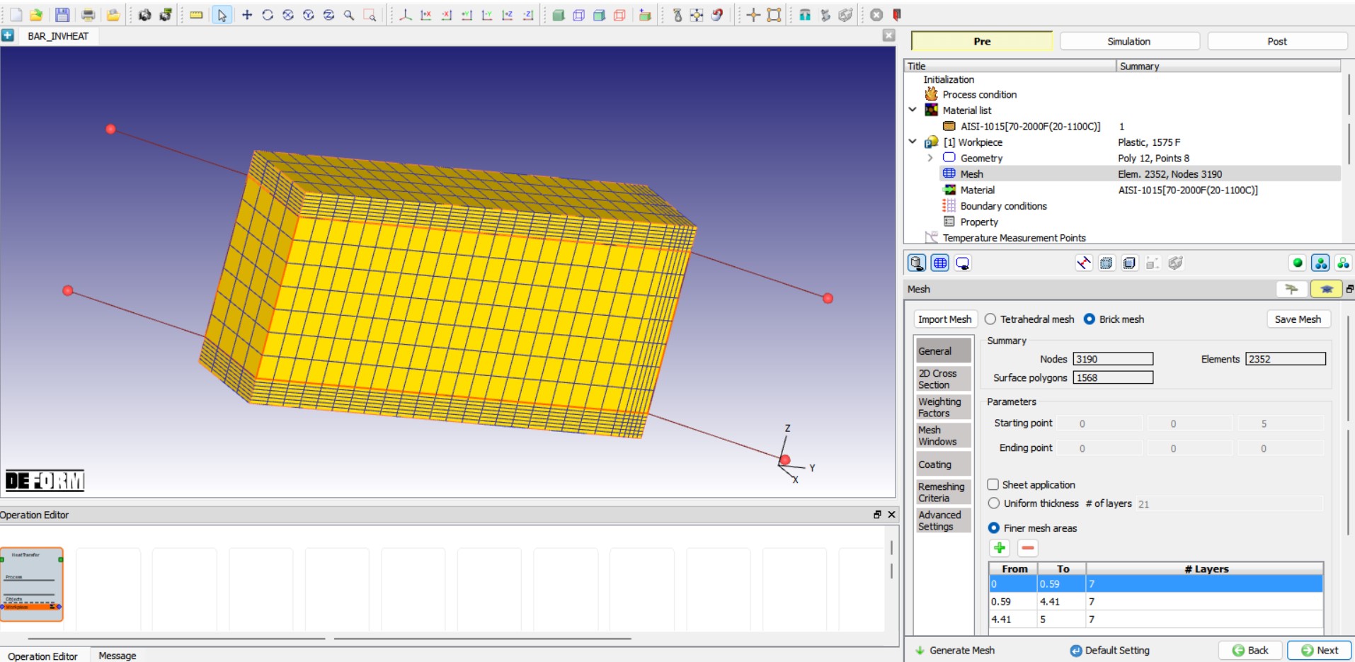
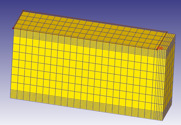
Generating mesh

Assigning Material

Select material “AISI-1015[70-2000F(20-1100C)] ” from the material list to assign to workpiece as shown in Fig. 3DINVL1.10. Click on to BCC page.

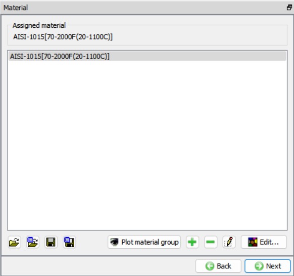
Assigning Material

BCC Definition

By default “Heat Exchange with Environment” should have been assigned to the non-symmetry faces of the object (see Fig. 3DINVL1.11.). Double check whether Heat Exchange with Environment BCC was applied. Manually apply the BCC to the non-symmetry faces if not already assigned. Click on until Temperature Measurement Points page.

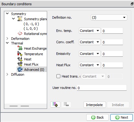
Heat Exchange BCC assigned for Workpiece

Temperature Measurement Points

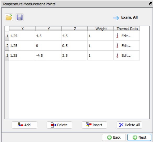
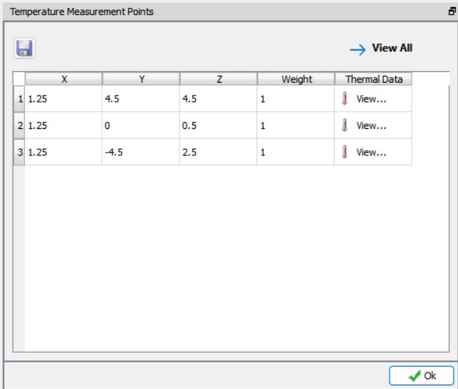
In “Temperature Measurement Points” page, click button three times and input coordinates (1.249, 4.5, 4.5), (1.249, 0, 0.5), and (1.249, -4.9, 2.5) in the table for point 1, 2, and 3, respectively as shown in Fig. 3DINVL1.12.

Thermal history data for each point can be defined by clicking on the button in the last column of the table. Click on and load “BAR_INVHEAT_Thermal_History_1.dat” file for point 1 from the /Labs folder and click button (see Fig. 3DINVL1.13.). Similarly load BAR_INVHEAT_Thermal_History_2.dat and BAR_INVHEAT_Thermal_History_3.dat for point 2 and 3 respectively. button in the last column of the table will change into after you had defined the Thermal History Data for the point. Click .

Note: If user want to define temperature measurement points for all the three points at a time, we can use button in Temperature Measurement Points page to load “BAR_INVHEAT_Thermal_History.DAT” from /Labs folder, all three points data is loaded into the wizard.

Temperature measurement Points page

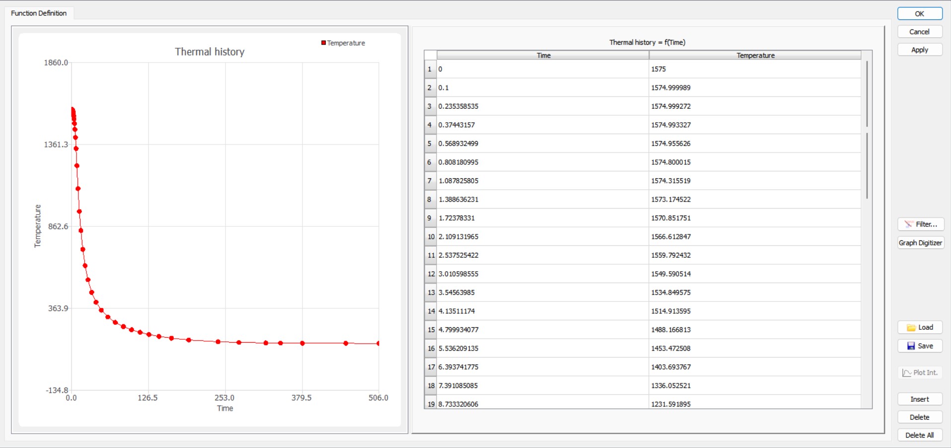
Thermal History Data window for Point 1

Defining Time Zones

In the time zones page, user can define time zones for Quenching and Transfer. Since in this lab we had opted to simulate only Transfer, only Transfer time zone definition is available. We would like to simulate the process for 506 sec as the last point of temperature measurement available from thermal history is at 506 sec. So enter Start time as 0sec and End time as 506 sec. Thermal History graph of all the points within the specified time can be seen in display area, see Fig. 3DINVL1.14. Click .

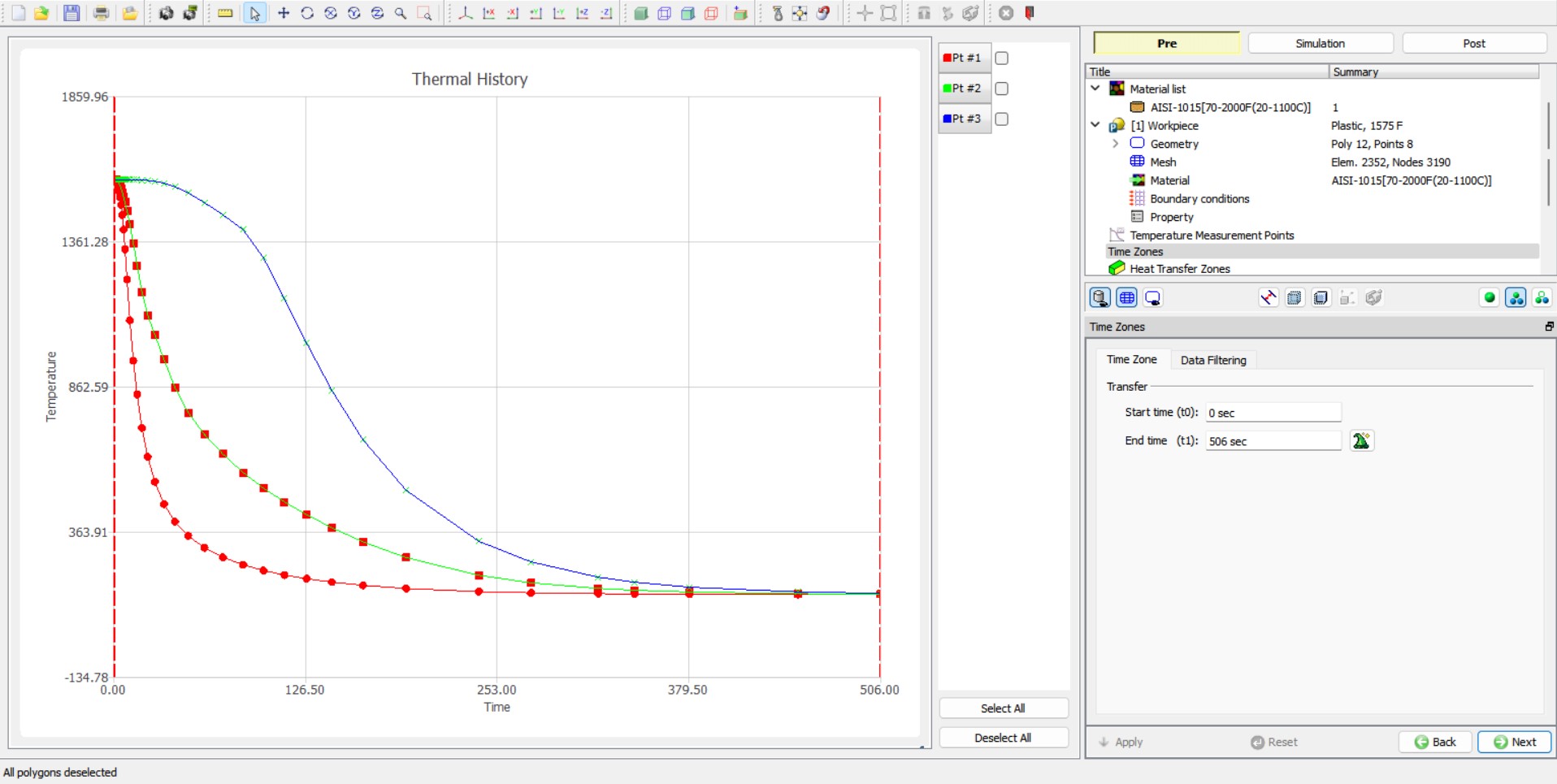
Transfer Time Definition in Time Zone Page

Defining Heat Transfer Zones

In “Heat Transfer Zones” page”, click twice to create two zones. To define each heat transfer zone, first select the appropriate row in the table and then pick surfaces on the object. (You may need to use in the picking options in the lower tool bar in order to achieve ideal picking results.) Select Zone #1 in the table and pick the faces normal to the -X, +Y and +Z directions to assign them to Zone #1(see Fig. 3DINVL1.15.). Select Zone #2 in the table and pick the face normal to the -Z direction to assign it to Zone #2 (see Fig. 3DINVL1.16.).

Note that the two symmetric planes are not included in any heat transfer zone.

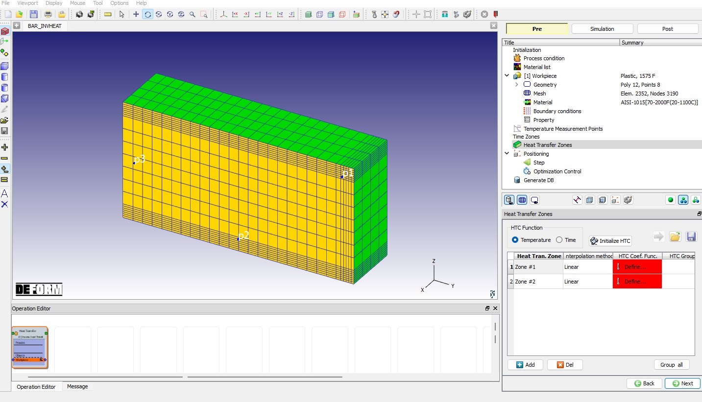
Defining Heat transfer Zone #1

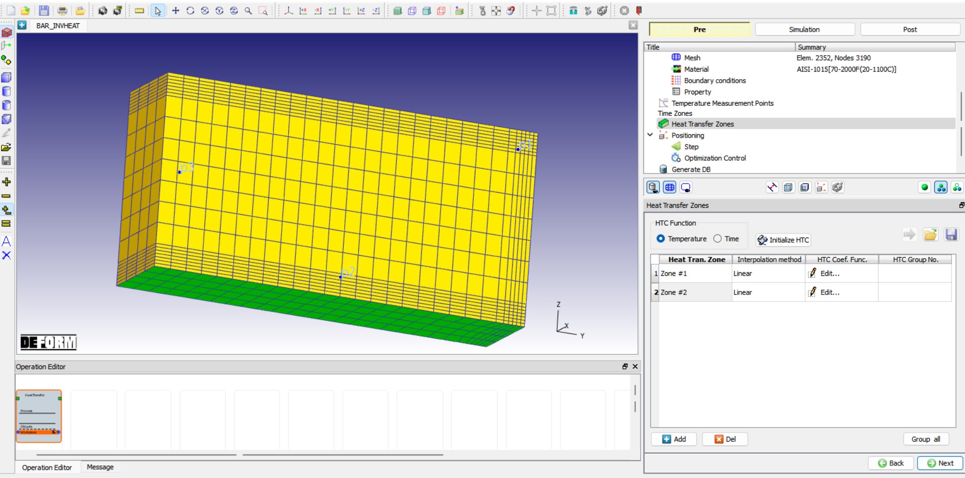
Defining Heat transfer Zone #2

After defining Heat transfer zone, click on button to define control points and limits, make sure HTC function is based on temperature. System adds control points by default, we will delete them for this lab and use six manually defined points. Click on the button to clear the table. Enter the following six values: 100, 400, 700, 1000, 1300, and 1600 as shown in Fig. 3DINVL1.17. Make sure interpolation method is Linear and initial guess, lower and upper bounds are fine. Click on button and then click on to close the Initializing Window.

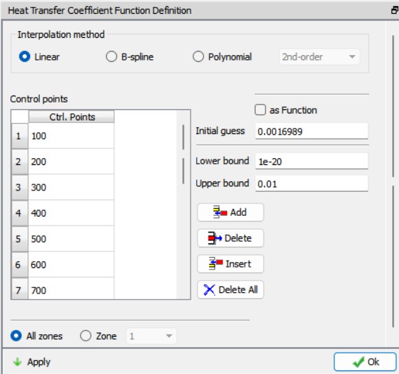
Defining Heat Transfer Coeffecient Function Definition

Control points and limits settings can be set for each zone separately using the button next to Zone in “Heat Transfer Zones” page, see Fig. 3DINVL1.15. Click on until “Step” page.

Defining Step controls

In “Step” page, keep “Temperature change per step” set as 1.8F and leave other values to defaults as shown in Fig. 3DINVL1.18. Click .

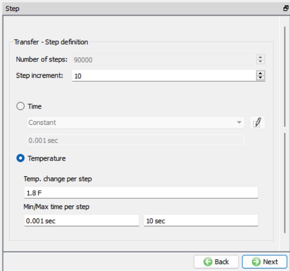
Defining Step controls

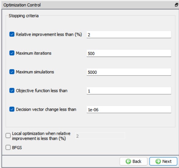
Optimization control

In “Optimization Control” page, as shown in Fig. 3DINVL1.19. make sure BFGS check box is in unchecked status. Click .

Optimization control Window

Database Generation

In DB Generation page, click on to verify the set up for errors and warnings, you should see a message “Data Valid!” if there are no errors. Click on to generate Database.

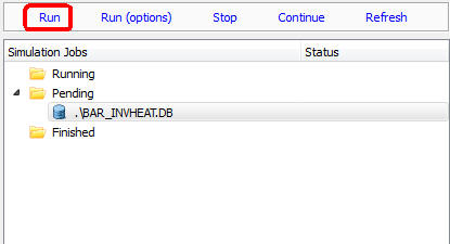
Optimization

After Database is generated, switch to tab above the object tree and click on button to start the optimization, see Fig. 3DINVL1.20. You can see a message “MULTIPLE OPERATION COMPLETED.” at the end of Simulation Log file after optimization is completed.

Running Optimization

Optimization results

To view optimization results, click on tab next to tab. In “Post Tools” page under “Tools” you can see two icons (see Fig. 3DINVL1.21.),

To view Optimized HTC values.

To view simulated temperature values at Temperature Measurement Points.

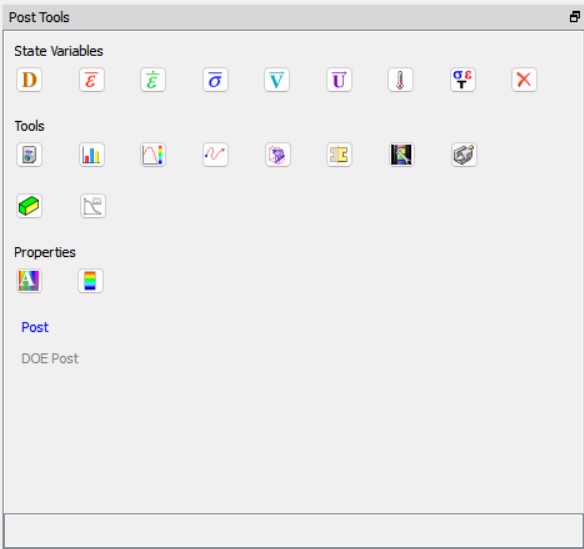
Post Tools to view Optimization Results

Click on to view optimized HTC values for each zone, a Heat Transfer Zone window will open as shown in Fig. 3DINVL1.22. Select each zone and click on view to observe the optimized HTC values, see Fig. 3DINVL1.23. shows Zone #1 optimized HTC values.

can be used to view objective value history, see Fig. 3DINVL1.24.

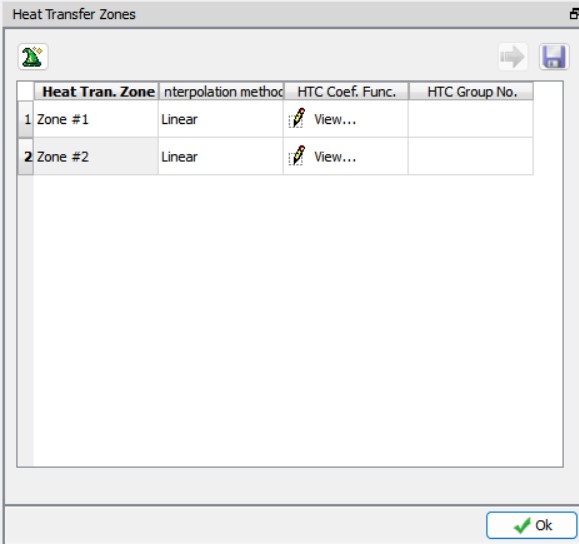
Heat Transfer Zones Window in Post Tab.

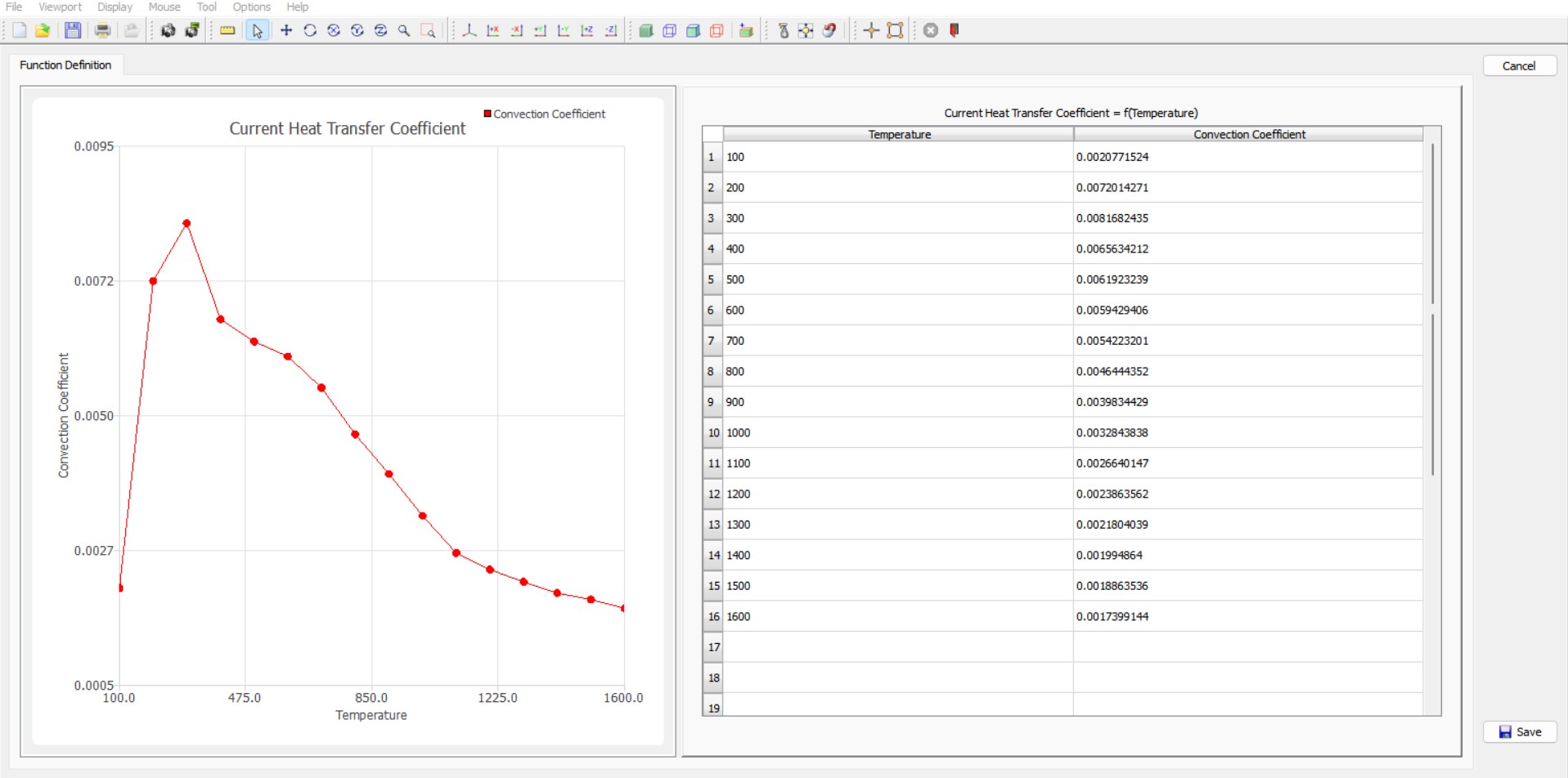
Optimized HTC values for Zone #1.

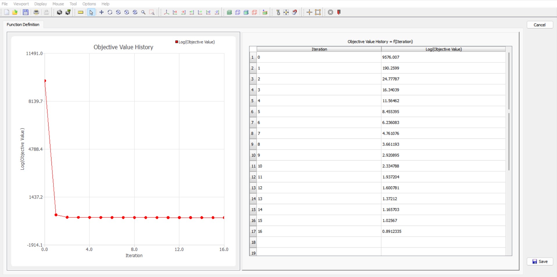
Objective Value History

The local objective optimization result can be viewed using , it gives the comparison between the experimental temperature and the simulated temperature values when the optimized heat transfer coefficient values are used. These values can be saved if necessary using button (see Fig. 3DINVL1.25.). User can select a point (see Fig. 3DINVL1.25.) and click on to plot the comparison between the experimental temperature and the simulated temperature values or to plot for all values, Fig. 3DINVL1.26. shows the comparison between the experimental temperature and the simulated temperature values for Point 1.

Temperature Measurement Points in Post

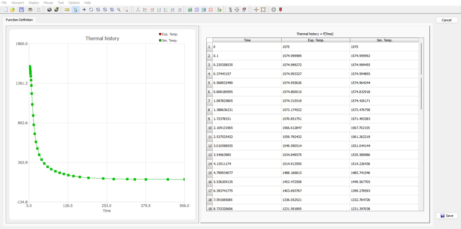
Local Objective Optimization Result for Point 1