2D Nitrocarburizing Lab1
Nitrocarburizing is a variation of the case hardening process. It is a thermochemical diffusion process where nitrogen, carbon, and to a very small degree, oxygen atoms diffuse into the surface of the steel part, forming a compound layer at the surface, and a diffusion layer. Nitrocarburizing is a shallow case variation of the nitriding process. This process is done mainly to provide an anti-wear resistance on the surface layer and to improve fatigue resistance.
This lab will demonstrate how to use MO template to prepare a Nitrocarburizing simulation.
1.1. Creating a New Problem
1.2. Adding Operation
1.3. Selecting Geometry Type
1.4. Simulation Controls
1.5. Adding material to the project
1.6. Define workpiece
1.6.1. Name the Object
1.6.2. Create Geometry
1.6.3. Assign Material for Workpiece
1.6.4. Mesh the Workpiece
1.7. Initialize Volume Fraction
1.8. Boundary Conditions
1.9. Stopping Controls
1.10. Step Controls
1.11. Generate Database
1.12. Running Simulation
1.13. Post Processing
Creating a New Problem
On a Windows machine, go to the ![]() button select DEFORM-v1x.xxx (.xxx indicates version number E.g. v14.0.2) and select DEFORM GUI Main v1x.x from the menu. The DEFORM GUI Main window will appear as shown in Fig. 2DNCL1.1.
button select DEFORM-v1x.xxx (.xxx indicates version number E.g. v14.0.2) and select DEFORM GUI Main v1x.x from the menu. The DEFORM GUI Main window will appear as shown in Fig. 2DNCL1.1.
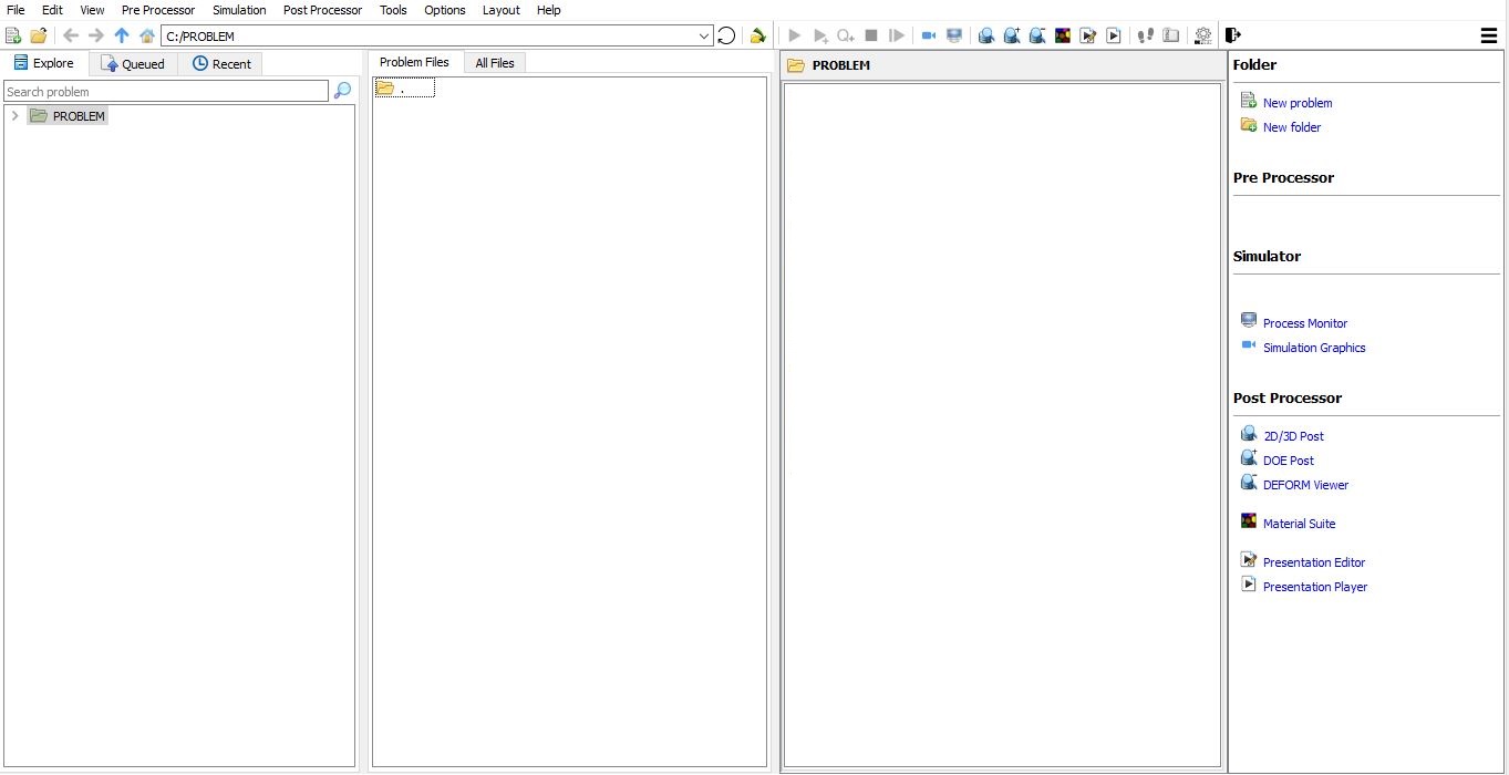
DEFORM GUI Main window
Create a new problem either by selecting File![]() **New Problem** or by clicking the New Problem
**New Problem** or by clicking the New Problem ![]() icon. The Problem Setup window will appear as shown in Fig. 2DNCL1.2. Select “ Integrated Manufacturing Process “ radio button and unit system as “SI “ radio button in unit field. Define Problem Name as “ 2D_Nitrocarburizng_Lab1 “ and make sure the “Show option dialog” check box is turned on (if we do not turn on the “Show option dialog ” check box, then we will not get the New Project dialog in MO UI). Then click on
icon. The Problem Setup window will appear as shown in Fig. 2DNCL1.2. Select “ Integrated Manufacturing Process “ radio button and unit system as “SI “ radio button in unit field. Define Problem Name as “ 2D_Nitrocarburizng_Lab1 “ and make sure the “Show option dialog” check box is turned on (if we do not turn on the “Show option dialog ” check box, then we will not get the New Project dialog in MO UI). Then click on ![]() button to open a new Problem using the Deform Integrated Manufacturing Process.
button to open a new Problem using the Deform Integrated Manufacturing Process.
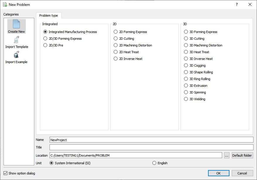
New Problem page
Multiple operation wizard will open with the New Project dialog, at this point user will be prompted to specify a project name (system will create a separate folder with this project name) and title for this session. In this session we will use “2D_Nitrocarburizng_Lab1 “ as the project name. Click on ![]() to continue to open the operation.
to continue to open the operation.
Adding Operation
Add 2D Forming operation from operations explorer list. Add the operation by clicking on ![]() button available next to 2D Forming or can also be added by drag and drop into the Operation editor (See Fig. 2DNCL1.3.). When we add the 2D Forming operation, process settings Window will open by default.
button available next to 2D Forming or can also be added by drag and drop into the Operation editor (See Fig. 2DNCL1.3.). When we add the 2D Forming operation, process settings Window will open by default.
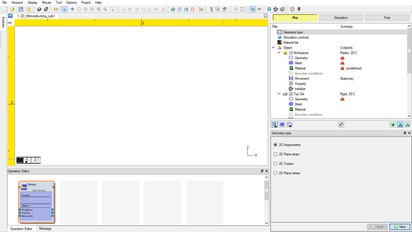
Adding 2D Forming operation
Click on the operation item the name tag, change it from ‘Forming’ to ‘Nitrocarburizing ’.
Selecting Geometry Type
Turn on ‘2D Plane strain ’ radio button in geometry type page (See Fig. 2DNCL1.4.), then click on ![]() to Simulation controls.
to Simulation controls.
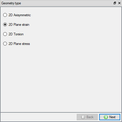
Geometry type selection
Simulation Controls
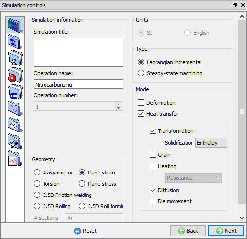
In this lab, we will be demonstrating how to setup Nitrocarburizing controls, Switch to ![]() mode as we need to use few advanced settings, in ‘Simulation controls’ window make sure ‘Diffusion ’ and ‘Transformation ’ under models ‘Heattransfer ’ are checked (See Fig. 2DNCL1.5.). Then click on
mode as we need to use few advanced settings, in ‘Simulation controls’ window make sure ‘Diffusion ’ and ‘Transformation ’ under models ‘Heattransfer ’ are checked (See Fig. 2DNCL1.5.). Then click on ![]() ‘Process conditions ’ page.
‘Process conditions ’ page.
Simulation control window
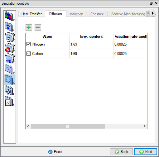
Nitrocarburizing is a variation of the nitriding process. It is a thermochemical diffusion process where nitrogen and carbon diffuse into the surface of the steel part, forming a compound layer at the surface, and a diffusion layer. To setup diffusion of both nitrogen and carbon, click on “Process condition “ then ‘Diffusion ’ tab. By default, ‘Carbon ’ is the only one atom showing here. Now click on ![]() to add another atom. For convenience, rename the first atom’s name to ‘Nitrogen ’, and the second to ‘Carbon ‘ , See Fig. 2DNCL1.6. Then click
to add another atom. For convenience, rename the first atom’s name to ‘Nitrogen ’, and the second to ‘Carbon ‘ , See Fig. 2DNCL1.6. Then click ![]() . Click
. Click ![]() in popup.
in popup.
Process Conditions – Diffusion of Multiple Atoms
Adding material to the project
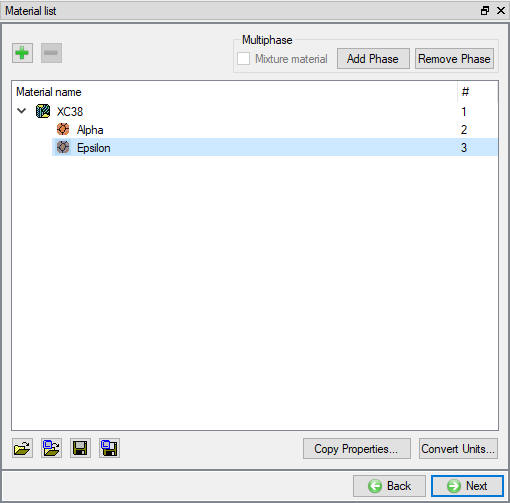
In ‘Material list’ window click on ![]() to add a new material, rename it to ‘XC38 ’. In this lab, a monolayer
to add a new material, rename it to ‘XC38 ’. In this lab, a monolayer  will form on XC38 substrate. Check ‘Multiphase ‘
 ![]() ‘Mixture material ’ and then add two phases: Alpha and Epsilon(See Fig. 2DNCL1.7.).
‘Mixture material ’ and then add two phases: Alpha and Epsilon(See Fig. 2DNCL1.7.).
Material List Window
The nitrogen contents (solubility limits) at the material interface are listed in table1.
| Position | N Content (Wt. %) | C Content (Wt. %) |
|---|---|---|
| Surface | 8 | 1 |
/  |
5.6 | - |
| / |
0.1 | - |
Nitrogen & Carbon contents
Click ![]() , comes to the first defined XC38 ’s material page. In this Nitrocarburizing lab, properties like phase transformation and diffusion coefficient need to be specified. Beware that, the diffusion coefficients of nitrogen and carbon need to be defined separately.
, comes to the first defined XC38 ’s material page. In this Nitrocarburizing lab, properties like phase transformation and diffusion coefficient need to be specified. Beware that, the diffusion coefficients of nitrogen and carbon need to be defined separately.
Transformation
To add the phase transformation relationships for XC38, click ![]() . Then from the mother phase choose ‘Alpha ’, and child phase ‘Epsilon ’, click
. Then from the mother phase choose ‘Alpha ’, and child phase ‘Epsilon ’, click ![]() to add the relationship. Under ‘Kinetics’ tab, select ‘Diffusion (Solubility curve)’ from the pull-down list to specify the model for the transformation (See Fig. 2DNCL1.8.).
to add the relationship. Under ‘Kinetics’ tab, select ‘Diffusion (Solubility curve)’ from the pull-down list to specify the model for the transformation (See Fig. 2DNCL1.8.).
The nitrided layer growth of follow a parabolic law, select the following model for the layer (Alpha ![]() Epsilon)
Epsilon)

type in 0.000132087 for the ‘Parabolic growth constant’ K. Then define nitrogen content ‘Start’ value of 0.4, and ‘End’ value 5.6, (See Fig. 2DNCL1.8.). Beware that the transformation relationship is defined for nitrogen, which is presented under the atom list  and was selected by default.
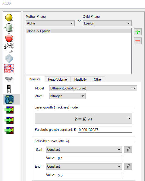
‘Material Editor’ - transformation definition
Diffusion Coefficient
The diffusion coefficients of Nitrogen in and phases are listed in Table 2, click the icon ![]() on the material page to define these settings for the corresponding materials.
on the material page to define these settings for the corresponding materials.
| Nitrocarburizing Temperature [°C] | 570 | |
|---|---|---|
| Diffusion Coefficient of Nitrogen [10-8mm2/s] | Epsilon () |
3.4 |
| Alpha () |
983.3 |
Diffusion coefficient of nitrogen

Diffusion Coefficient of Nitrogen - Alpha
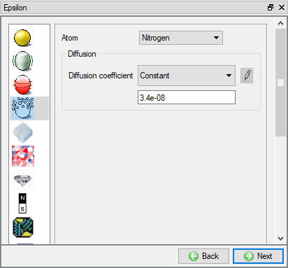
Diffusion Coefficient of Nitrogen - Epsilon
The diffusion coefficients of Carbon in and phases are listed in Table 3, click the icon ![]() on the material page to define them for the corresponding materials. Beware to choose the carbon from the atom list
on the material page to define them for the corresponding materials. Beware to choose the carbon from the atom list 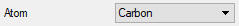 , see Fig. 2DNCL1.11. and Fig. 2DNCL1.12.
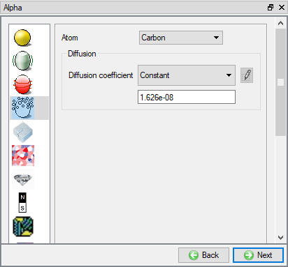
Diffusion Coefficient of Carbon - Alpha
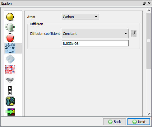
Diffusion Coefficient of Carbon - Epsilon
| Nitrocarburizing Temperature [°C] | 570 | |
|---|---|---|
| Diffusion Coefficient of Nitrogen [10-8mm2/s] | Epsilon () |
883.3 |
| Alpha () |
1.626 |
Diffusion coefficient of carbon
Thermal Properties
Thermal properties are not necessary because the object’s temperature is constant and same as the environment temperature in this lab. But they are still required for DB generation. For XC38, type 30 for thermal conductivity, 5.5 as heat capacity, 0.7 as emissivity and 7.85e-09 as density, see Fig. 2DNCL1.13. Then Type in the same values for all the child materials.
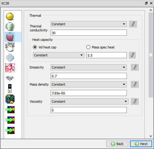
Thermal Properties Page
Define workpiece
Click on the ‘Object ’ item from the operation tree, go to object list page. From the list, delete all the other objects except the ‘Workpiece’.
Name the Object
Click on the ‘Workpiece ‘ item from operation tree, go to define the object. Type in ‘XC38 specimen’ as object name, set the temperature to 570 °C, and leave all others as default (See Fig. 2DNCL1.14.). Then click on ![]() go to the ‘Geometry ‘ definition page.
go to the ‘Geometry ‘ definition page.
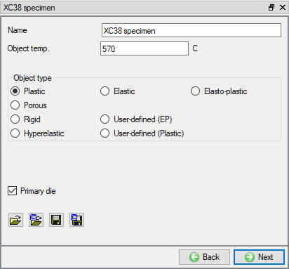
Workpiece definition page
Create Geometry
In ‘Geometry’ page, click on ![]() , on the following page choose ‘Bar ‘, and give 13 mm as width , 13 mm as height and (-6.5, -6.5) as center X, Y (See Fig. 2DNCL1.15), the object geometry is also previewed at the central graphic window area. Click on
, on the following page choose ‘Bar ‘, and give 13 mm as width , 13 mm as height and (-6.5, -6.5) as center X, Y (See Fig. 2DNCL1.15), the object geometry is also previewed at the central graphic window area. Click on ![]() button to accept all the changes, and it will come back to the ‘Geometry’ definition. Click on
button to accept all the changes, and it will come back to the ‘Geometry’ definition. Click on ![]() until Material page to assign material.
until Material page to assign material.
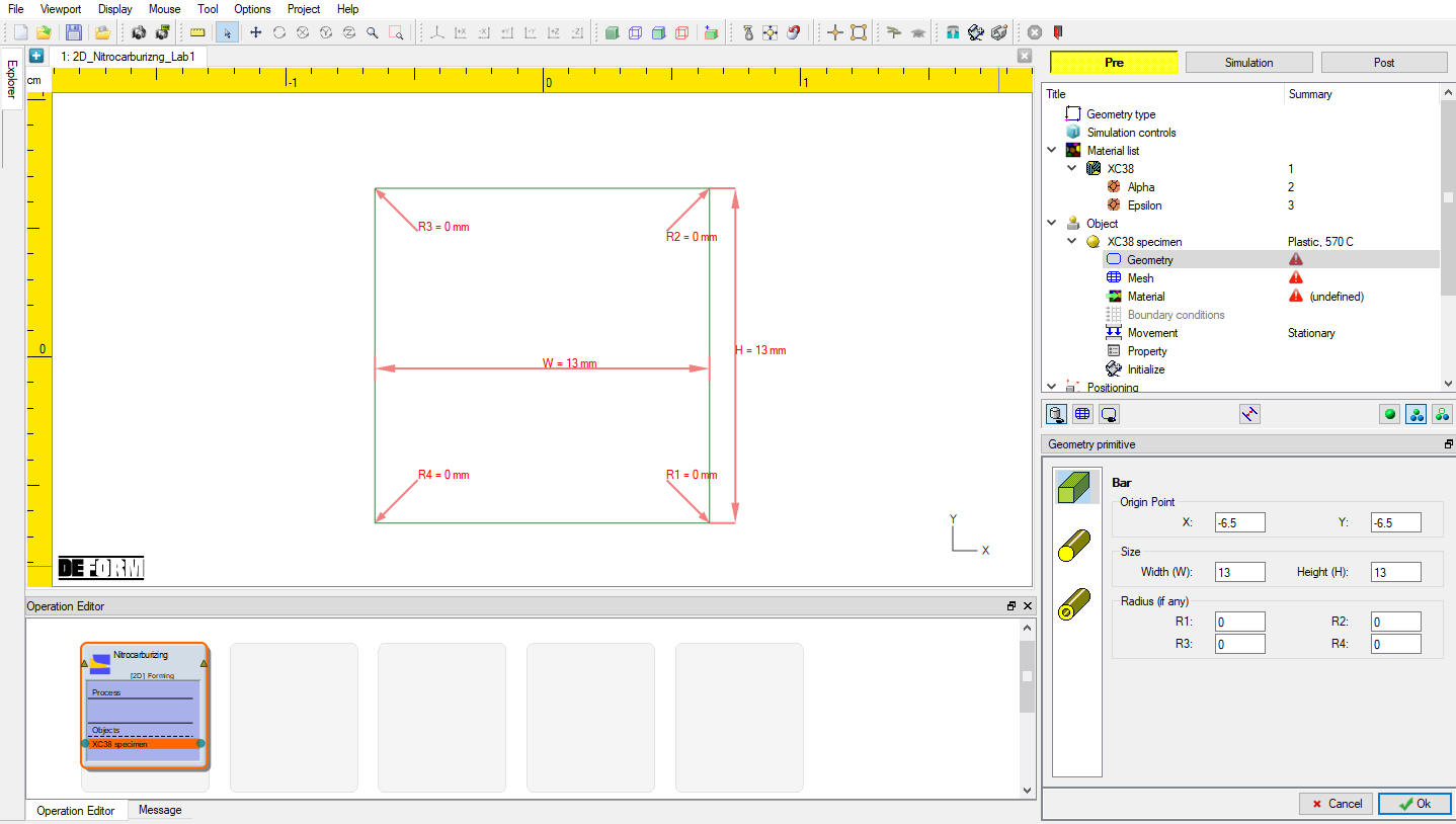
Geometry primitive to create the specimen part
Assign Material for Workpiece
Assign “XC38 “ material from list for workpiece and click on ![]() to Mesh page.
to Mesh page.
Mesh the Workpiece
In this lab simulation, the total thickness of the compound layer is about 40m, coating mesh is suggested to represent the compound layer. And mesh window is also used to create finer surface mesh layer. On ‘General ’ mesh page, keep default ‘System setup’ option, put 1600 in ‘Target number of Elements ‘ (See Fig. 2DNCL1.16.). Then click on ‘Weighting Factors ‘, increase the weight of ‘Meshwindows ’ to 0.8, See Fig. 2DNCL1.17.
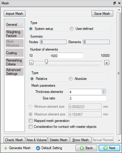
General Mesh page
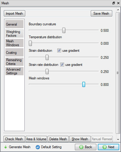
Weighting Factors
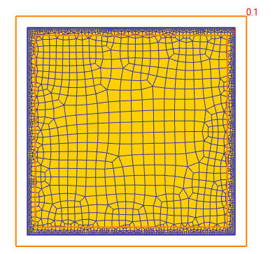
Next click on ‘Mesh Windows ‘, create two rectangle mesh windows. The first window is put inside the object with relative element size of1 , and second window covers the entire workpiece with the relative element size of 0.1 (see Fig. 2DNCL1.18.), this will result into finer surface mesh layer.
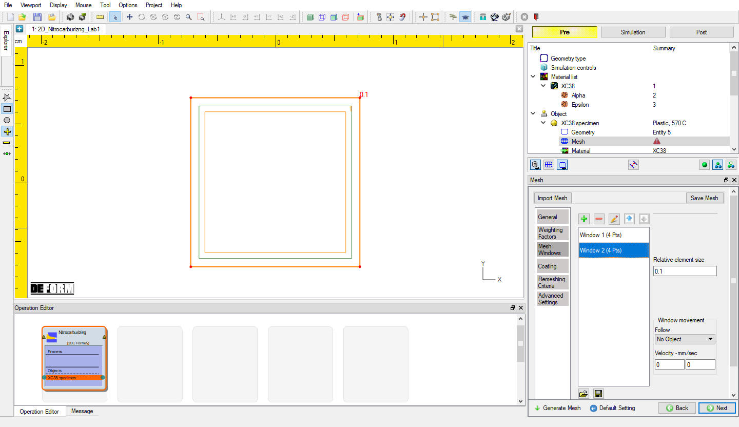
Mesh Windows Defined for Workpiece
Next to define coating layer, click on ‘Coating ‘, add 12 coating layers of varied thickness as shown in Fig. 2DNCL1.19.
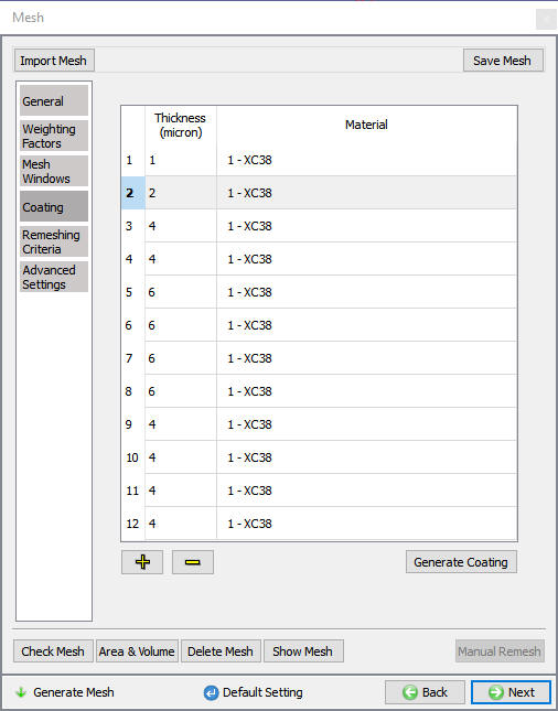
Coating Layers for Workpiece
Now click on ![]() to generate the mesh. Click
to generate the mesh. Click ![]() on the pop-up windows to continue. The mouse icon on the screen turns to busy and then back to normal, which indicates that the mesh has been generated, the results are also plotted on the central graphic area, see Fig. 2DNCL1.20.
on the pop-up windows to continue. The mouse icon on the screen turns to busy and then back to normal, which indicates that the mesh has been generated, the results are also plotted on the central graphic area, see Fig. 2DNCL1.20.
Mesh Generation
Initialize Volume Fraction
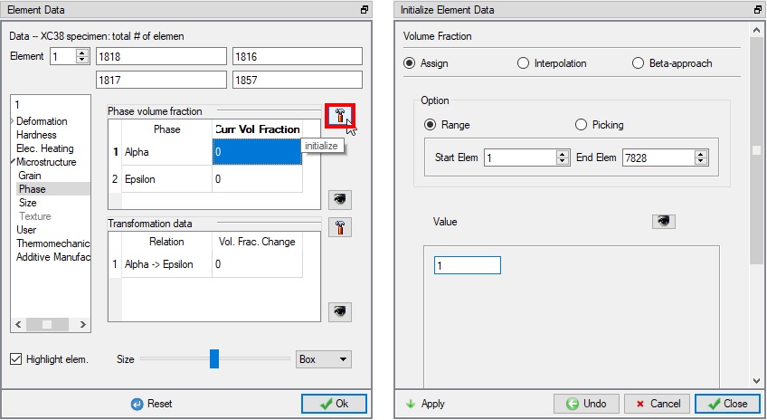
At this moment, click on ![]() to access to the element dialog to initialize the volume fraction. On the item list window click ‘Microstructure’
to access to the element dialog to initialize the volume fraction. On the item list window click ‘Microstructure’![]() ‘Phase’. Then choose ‘Alpha ’ and click on
‘Phase’. Then choose ‘Alpha ’ and click on ![]() to ‘Initialize Element Data’. Type in 1 , then click on
to ‘Initialize Element Data’. Type in 1 , then click on ![]() , then close the window. click
, then close the window. click ![]() until BCC page.
until BCC page.
Element Dialog – Initialization of Phase Volume
Boundary Conditions
Heat Exchange with Environment
It can be seen that ‘Heat Exchange with Environment’ BCC has been already defined on the entire object surface when mesh was generated. Click on “Defined” , then “Environment “ to change the ‘Environmenttemperature ’ to 570 °C, which is same as the object temperature ( Fig. 2DNCL1.22.).
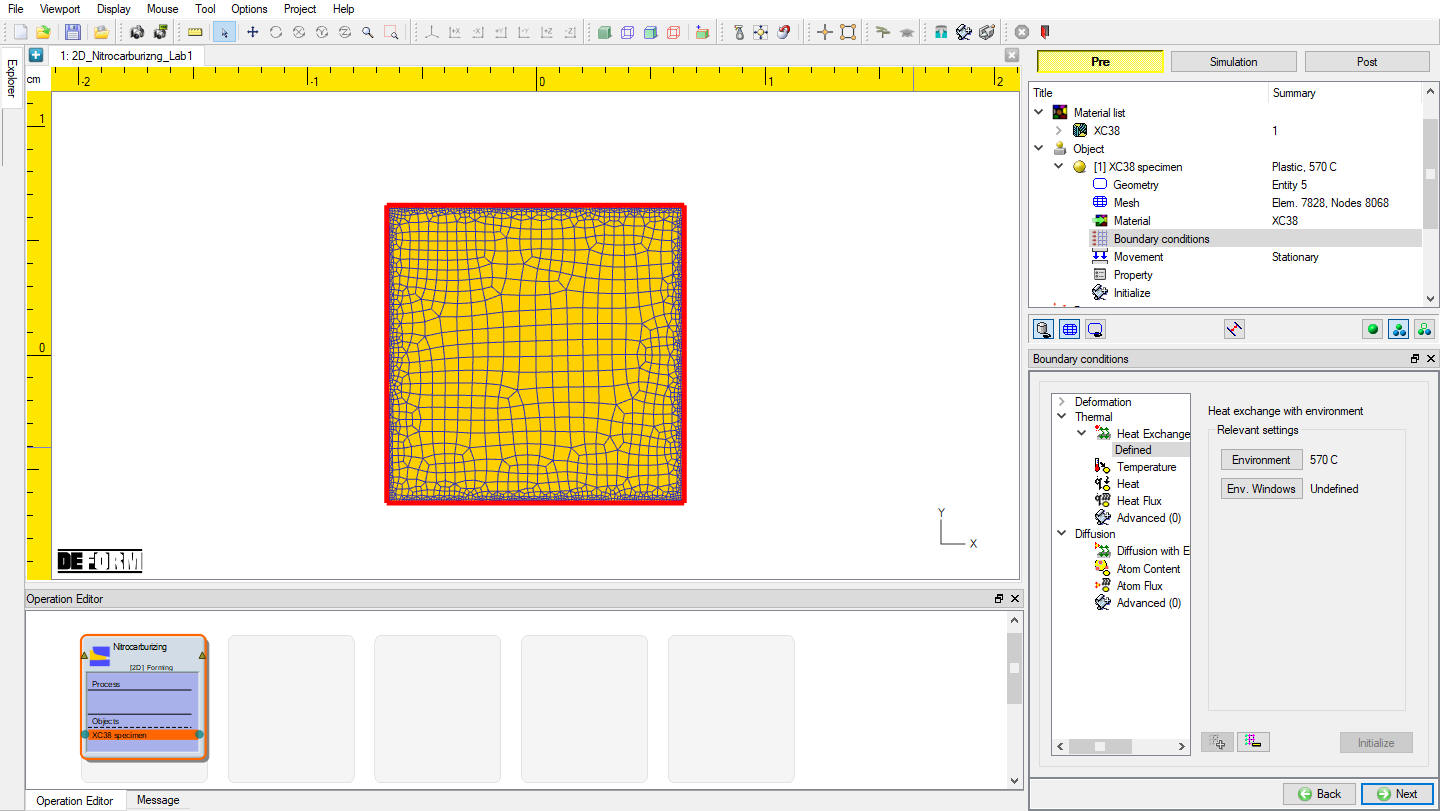
Heat Exchange with Environment Definition
Diffusion BCC
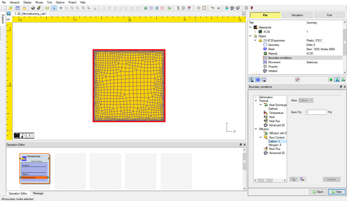
Constant Nitrogen contents on the workpiece are assumed in this Nitriding Lab simulation, to do so make sure Nitrogen is selected from the atom list and click on ‘Atom content’. Then type in 8 for the ‘AtomPct. ’. Select the entire object surface by clicking on ![]() on the picking dialog, then click on
on the picking dialog, then click on ![]() to finish the assignment. The BCC definition can be seen in Fig. 2DNCL1.23.
to finish the assignment. The BCC definition can be seen in Fig. 2DNCL1.23.
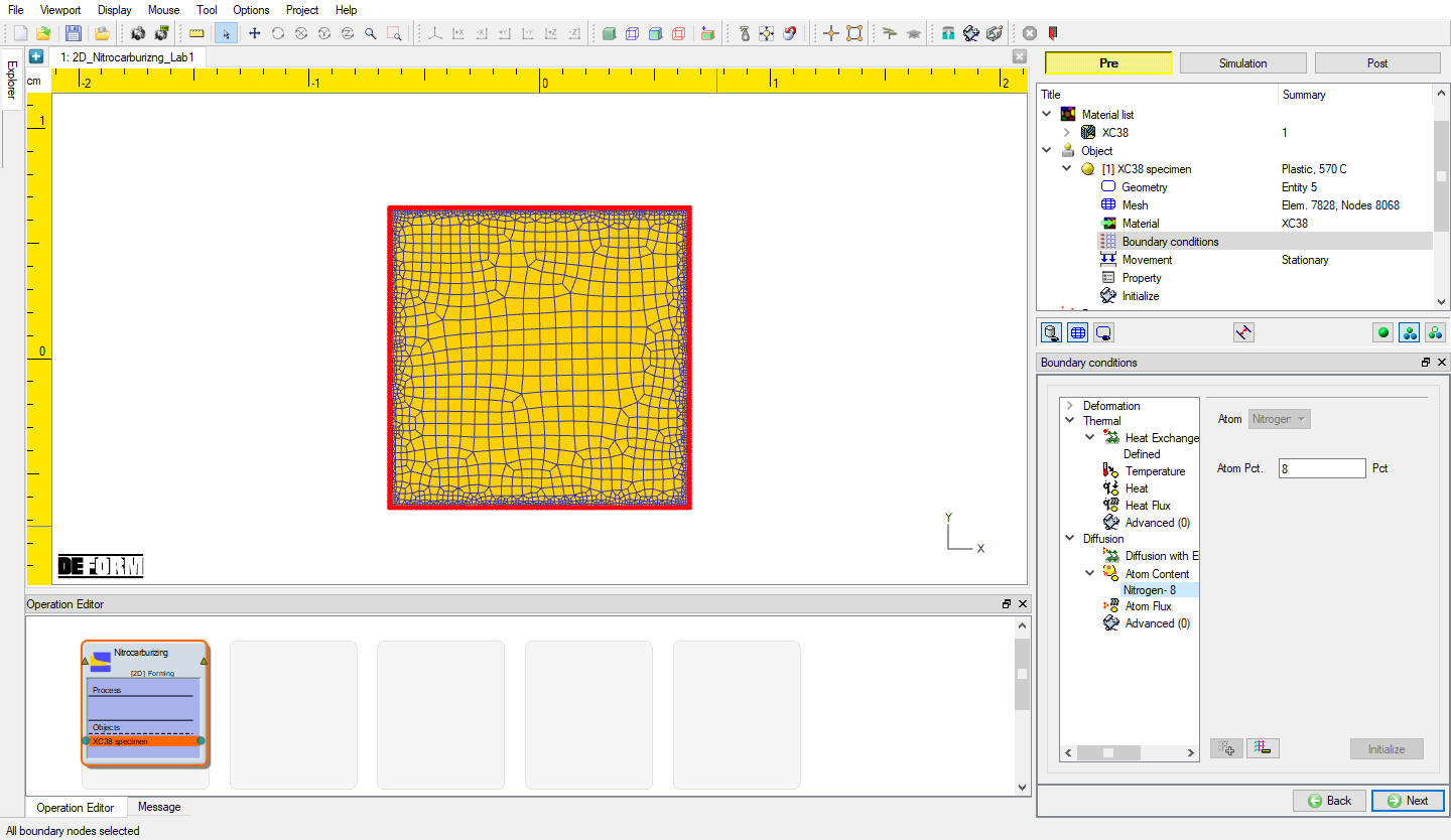
Constant Nitrogen Surface Content
Also, constant Carbon contents on the workpiece are assumed. Click on ‘Atom content ‘, choose ‘Carbon’ from the ‘Atom’ list , Then type in 1 for the ‘AtomPct. ’. Select the entire object surface by clicking on ![]() icon on the picking dialog, then click on
icon on the picking dialog, then click on ![]() (See Fig. 2DNCL1.24.). Click
(See Fig. 2DNCL1.24.). Click ![]() until Stopping controls page.
until Stopping controls page.
Constant Carbon Surface Content
Stopping Controls
Go to define the process duration. Make sure the system is in ‘Expert’ mode, if not, click on ![]() will switch the system to the expert mode. Then type in 108000 in the ‘Process duration ’ field, see Fig. 2DNCL1.25. Then click on
will switch the system to the expert mode. Then type in 108000 in the ‘Process duration ’ field, see Fig. 2DNCL1.25. Then click on ![]() to ‘Step’ controls page.
to ‘Step’ controls page.
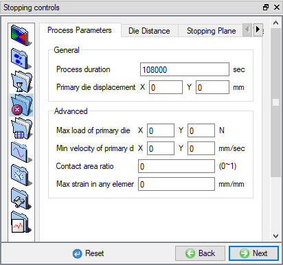
Stopping Controls (Expert Mode)
Step Controls
Switch back to the ‘Guide’ mode by clicking on ![]() , Since process duration has been defined simulation will stop accordingly,, type 999999 into ‘Numberof steps ’ field. Set 5 as ‘Stepincrement ’ and 20 sec. as the time per step(see Fig. 2DNCL1.26.). Then click on
, Since process duration has been defined simulation will stop accordingly,, type 999999 into ‘Numberof steps ’ field. Set 5 as ‘Stepincrement ’ and 20 sec. as the time per step(see Fig. 2DNCL1.26.). Then click on ![]() to ‘Generate DB’ page.
to ‘Generate DB’ page.
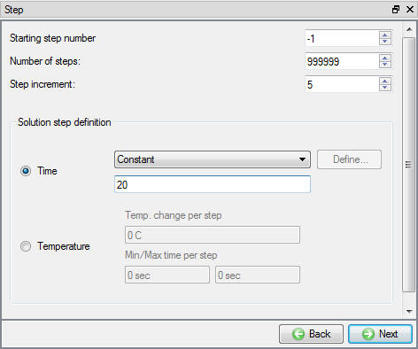
Step Controls (Guide Mode)
Generate Database
In ‘Generate DB’ page, click ![]() to see if anything was missed in the setup and then click on the
to see if anything was missed in the setup and then click on the ![]() button to generate the database. Observe the message in Message tab informing database generation status.
button to generate the database. Observe the message in Message tab informing database generation status.
Running Simulation
Once the database has been generated, switch to the Simulation mode by clicking on ![]() button above the operation tree. Click on the
button above the operation tree. Click on the ![]() action label to open the Run Options dialog as shown in Fig. 2DNCL1.27. Use the default Continue Run option to select “Continue from the last step ” (from step -1) option and then select the Simulation mode as Interactive and click on
action label to open the Run Options dialog as shown in Fig. 2DNCL1.27. Use the default Continue Run option to select “Continue from the last step ” (from step -1) option and then select the Simulation mode as Interactive and click on ![]() button to run the simulation.
button to run the simulation.
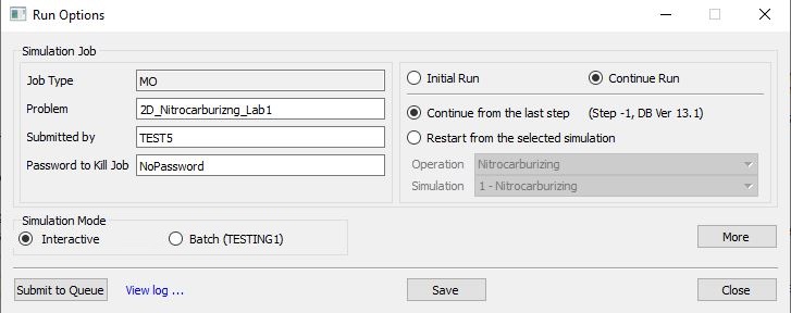
Run Simulation Window
Monitor the progress of the simulation by looking at the Simulation Message and Simulation Log tab, making sure that the ![]() option is checked. User can view the Nitrocarburizing process as the simulation proceeds to the specified Step definition from Simulation graphics.
option is checked. User can view the Nitrocarburizing process as the simulation proceeds to the specified Step definition from Simulation graphics.
Post Processing
After the simulation is finished, open the DB in Next Gen post - processor.
Nitrogen Profiles
‘State variables between two points’ function is a great tool to exam nitrogen concentration profile (vs. depth below the surface).
Click on ![]() , Under Diffusion
, Under Diffusion ![]() Dominant atom, select “ Nitrogen “ State variable and click on
Dominant atom, select “ Nitrogen “ State variable and click on ![]() to plot and click on
to plot and click on ![]() .
.
Go to last step, then click on State variables between two points ![]() to generate nitrogen profile. Define Start and End points and click on generate
to generate nitrogen profile. Define Start and End points and click on generate ![]() . Right click on State variable between two points graph and select “Set Graph Properties “, then select ‘Range’ page, set ‘Y Axis’ to ‘User-defined’, then define Min as 0.0 and Max as 8.0. values and click on
. Right click on State variable between two points graph and select “Set Graph Properties “, then select ‘Range’ page, set ‘Y Axis’ to ‘User-defined’, then define Min as 0.0 and Max as 8.0. values and click on ![]() button (see Fig. 2DNCL1.28.). Click
button (see Fig. 2DNCL1.28.). Click ![]() to close Property editor popup.
to close Property editor popup.
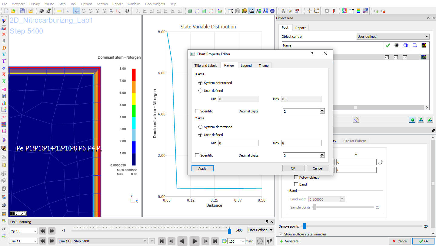
SV between 2 Points: Atom-Nitrogen
Carbon Profiles
Click on ![]() , Under Diffusion
, Under Diffusion ![]() Dominant atom, select “ Carbon “ State variable and click on
Dominant atom, select “ Carbon “ State variable and click on ![]() to plot and click on
to plot and click on ![]() (See Fig. 2DNCL1.29.).
(See Fig. 2DNCL1.29.).
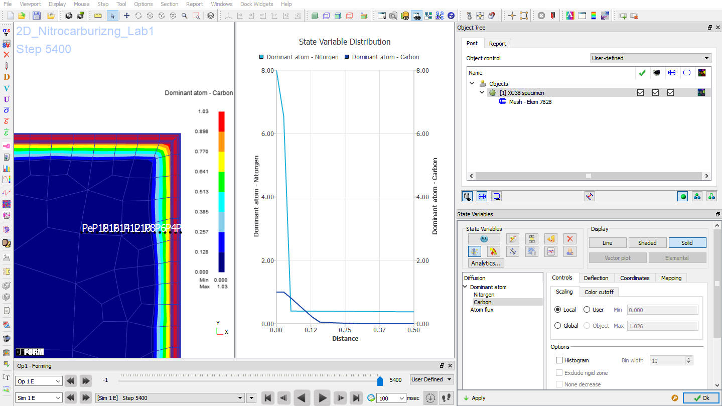
SV between 2 Points: Atom-Carbon