Lab 07 Mechanical Press
Requirement: To setup this operation, First we have to setup Lab 03 Spike Isothermal Lab.
7.1. Creating a New Problem
7.2. Adding Operation
7.3. Import Database
7.4. Assigning Top Die Movement
7.5. Generate Database
7.6. Starting the Simulation
7.7. Post-processing the Results
Creating a New Problem
On a Windows machine , go to the ![]() button select DEFORM-v1x.xxx (.xxx indicates version number E.g. v14.0.2) and select DEFORM GUI Main vxx.xx from the menu. The DEFORM GUI Main window will appear.
button select DEFORM-v1x.xxx (.xxx indicates version number E.g. v14.0.2) and select DEFORM GUI Main vxx.xx from the menu. The DEFORM GUI Main window will appear.
Create a new problem either by selecting File ![]() New Problem or by clicking the New Problem
New Problem or by clicking the New Problem ![]() icon. The Problem Setup window will appear. Select “Integrated Manufacturing Process “ radio button and unit system as “English “ radio button in unit field. Define Problem Name as “ **Spike_Mechanical** “ and make sure the “Show option dialog ” check box is turned on (if we do not turn on the “Show option dialog” check box, then we will not get the New Project dialog). Then click on
icon. The Problem Setup window will appear. Select “Integrated Manufacturing Process “ radio button and unit system as “English “ radio button in unit field. Define Problem Name as “ **Spike_Mechanical** “ and make sure the “Show option dialog ” check box is turned on (if we do not turn on the “Show option dialog” check box, then we will not get the New Project dialog). Then click on ![]() button to open a new problem using the Deform Integrated Manufacturing Process.
button to open a new problem using the Deform Integrated Manufacturing Process.
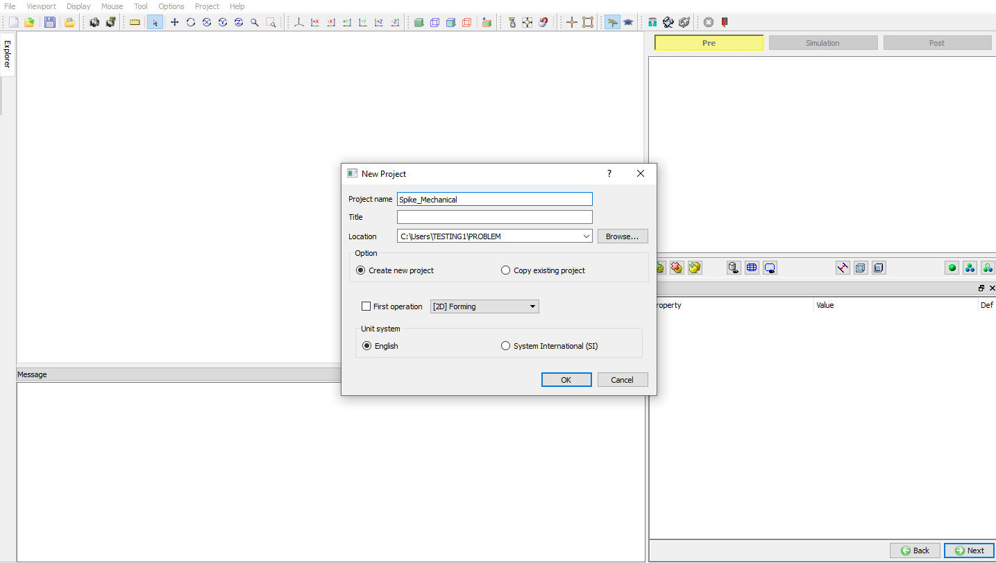
Multiple operation wizard will open with the New Project dialog (See Fig. L7.1.), at this point user will be prompted to specify a project name (system will create a separate folder with this project name) and title for this session. In this lab we use ‘Spike_Mechanical ’ as the project name.
Assigning Problem Name
User can also change the Unit system, project saving file location and add operation by selecting from First operation pull down list and checkbox (see Fig. L7.1.). Using copy Existing project option we can import previous saved projects as new project. Click on to continue to open the operation.
Adding Operation
Multiple Operation wizard will open. Add 2D Forming operation from the Explorer Operations list. Operation can be add by clicking on 2D Forming operation ![]() button or user can also add by drag and drop into the Operation Editor. (See Fig. L7.2.)
button or user can also add by drag and drop into the Operation Editor. (See Fig. L7.2.)
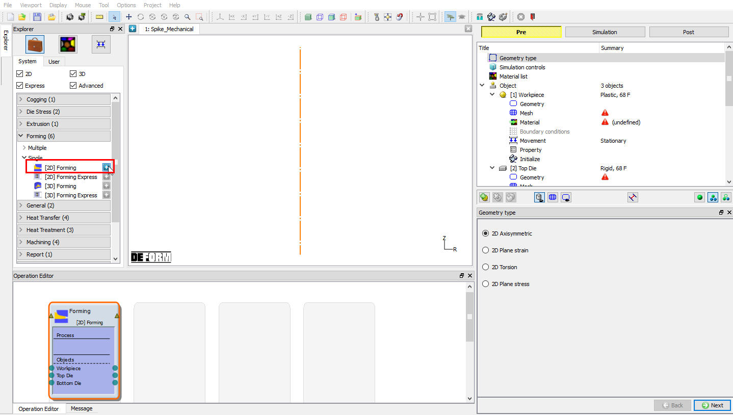
Add 2D Forming operation into Operation Editor
Import Database
Using Import option ![]() , Load the database of problem Spike_Isothermal , Select -1 step in the Step selection window (see Fig. L7.3.), then click on
, Load the database of problem Spike_Isothermal , Select -1 step in the Step selection window (see Fig. L7.3.), then click on ![]() .
.
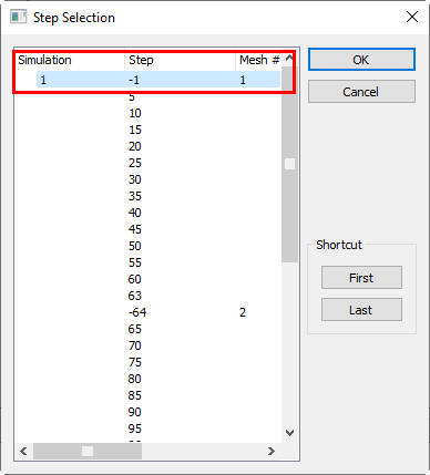
Selecting step in Step Selection window
In this lab we will assign Mechanical movement for Top die, click on ![]() until Top Die movement page.
until Top Die movement page.
Assigning Top Die Movement
Select Mechanical movement type, define Total stroke as 22.5 in, Forging stroke as 12 in and Cycle/sec as 1 (See Fig. L7.4.). Then click on ![]() until Generate DB page.
until Generate DB page.
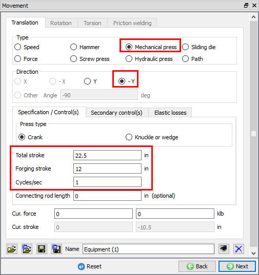
Top Die Movement Die page
Generate Database
Click the ![]() button to have the program check to see if anything was missed in the problem setup. During the checking process:
button to have the program check to see if anything was missed in the problem setup. During the checking process:
Messages in the red color signify data that needs to be fixed before a simulation can be run (such as when you forget to define any material data).
Click on ![]() button to generate the database. When the program is done writing the database, click on
button to generate the database. When the program is done writing the database, click on ![]() tab to run simulation.
tab to run simulation.
Starting the Simulation
Click on ![]() under the simulation tab (see Fig. L7.5.), as we click on the Run option, Run simulation dialog will open (see Fig. L7.6.), use the default Continue Run option to select “Continue from the last step ” option and then select the Simulation mode as Interactive and click on
under the simulation tab (see Fig. L7.5.), as we click on the Run option, Run simulation dialog will open (see Fig. L7.6.), use the default Continue Run option to select “Continue from the last step ” option and then select the Simulation mode as Interactive and click on ![]() button to run the simulation.
button to run the simulation.

Simulation Options

Run Simulation window
The progress of the simulation can be monitored as it is running by looking at the Simulation Message and Simulation Graphics in Simulation mode. Click the Simulation Message tab to view the Message file. As long as the ![]() option is checked, which is the default setting, the Message file will refresh every couple of seconds.
option is checked, which is the default setting, the Message file will refresh every couple of seconds.
The Message file provides information about which simulation step the simulation is currently on and also gives information dealing with how well the simulation is running.
When the simulation has finished, the following message will be added to the end of the Message file:”NORMAL STOP: Simulation is completed and stopped at the user specified time step”.
Post-processing the Results
After simulation has been completed, click on ![]() tab, MO post processor will open.
tab, MO post processor will open.
Load-Stroke Graph:
Plot Y-Speed v/s Stroke graph for Top die.
Click the ![]() icon, the Load Stroke Graph window will open. Select the Top Die in Plot object list, in X-Axis pull down menu select Stroke and in Y-Axis pull down menu select Y Speed. Click on options tab and check Step tracer check box, then click on
icon, the Load Stroke Graph window will open. Select the Top Die in Plot object list, in X-Axis pull down menu select Stroke and in Y-Axis pull down menu select Y Speed. Click on options tab and check Step tracer check box, then click on![]() . The Load Stroke graph will display on the right side of the display window (see Fig. L7.7.). When a different step is selected, the balloon in the Load-Stroke curve will highlight that step and the corresponding load for that step will be shown in the graph. Also, a point on the graph can be picked with the mouse and the displayed step will automatically change to the one corresponding to that point on the graph.
. The Load Stroke graph will display on the right side of the display window (see Fig. L7.7.). When a different step is selected, the balloon in the Load-Stroke curve will highlight that step and the corresponding load for that step will be shown in the graph. Also, a point on the graph can be picked with the mouse and the displayed step will automatically change to the one corresponding to that point on the graph.

Y-Speed Stroke Graph plot
Similarly plot Y-Load v/s Stroke graph for Top die and observe the graph. (See Fig. L7.8.)

Y-Load Stroke graph plot
After completion of Post processing, Save the Project and close the MO wizard by clicking Close ![]() button or selecting Quit option under File menu.
button or selecting Quit option under File menu.
Related Topics: