2D DOE Lab1

In this lab we import the Multi Stand Drawing setup keyfile from 2D labs and then continue with the nominal project simulation and DOE setup.

1.1. Nominal Project setup and simulation

1.2. Check and define the Nominal Project

1.3. Add DOE Project

1.4. Add die geometry variation as DOE variable

1.5. Add Friction coefficient as DOE variable

1.6. Check DOE Variables table

1.7. DOE Samples definition

1.8. Define DOE Output operation

1.8.1. Select DOE Operation and object to Study

1.8.2. Define Output variables

1.9. Simulate DOE project

1.10. Review the DOE results

1.10.1. Check Operation min/max (all steps) variables

1.10.2. Check Summary min/max (last step) variables

1.10.3. Check Location specific (One step) variables

Nominal Project setup and simulation

On a Windows machine , go to the button select DEFORM-v1x.xxx (.xxx indicates version number E.g. v14.0.2) and select DEFORM GUI Main vxx.xx from the menu. The DEFORM GUI Main window will appear.

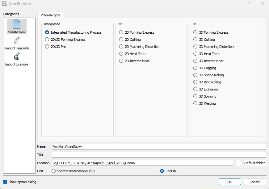
Create a new problem either by selecting File New Problem or by clicking the New Problem icon. The Problem Setup window will appear as shown in Fig. DOEL1.1. Select “Integrated Manufacturing Process “ radio button and unit system as “English “ radio button in unit field. Define Problem Name as “ DoeMultiStandDraw “ and make sure the “Show option dialog” check box is turned on (if we do not turn on the “Show option dialog ” check box, then we will not get the New Project dialog in MO UI). Then click on button to open a new Problem using the Deform Integrated Manufacturing Process.

New Problem page

Integrated Manufacturing Process will open, at this point user will be prompted to specify a project name (system will create a separate folder with this project name) and title for this session. In New Project popup define Problem Name as ‘DoeMultiStandDraw ‘, select First Operation as 2D Forming and select English unit system as shown in Fig. DOEL1.2. , click on to add project.

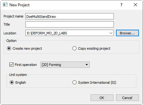
New Project creation window

Click on (Import DB/Keyfile) icon and import MultiStandDraw.key file from installation path 2D/LABS folder as shown in Fig. DOEL1.3.

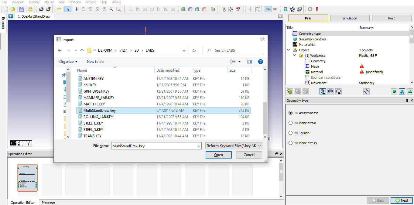
Importing Nominal project setup keyfile

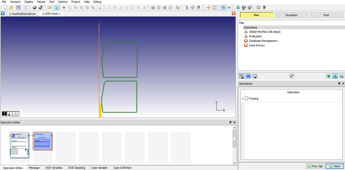
After importing the keyfile MO will display all objects as shown in Fig. DOEL1.4.

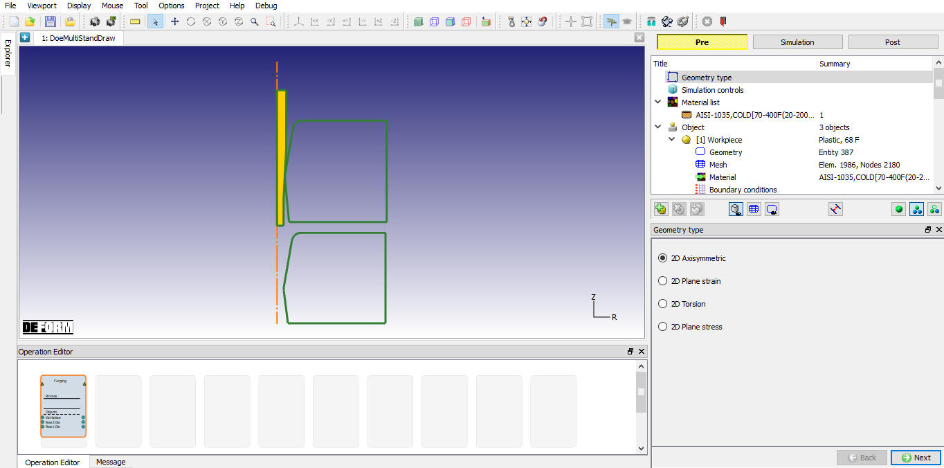
MO project layout after importing the setup keyfile

Check and define the Nominal Project

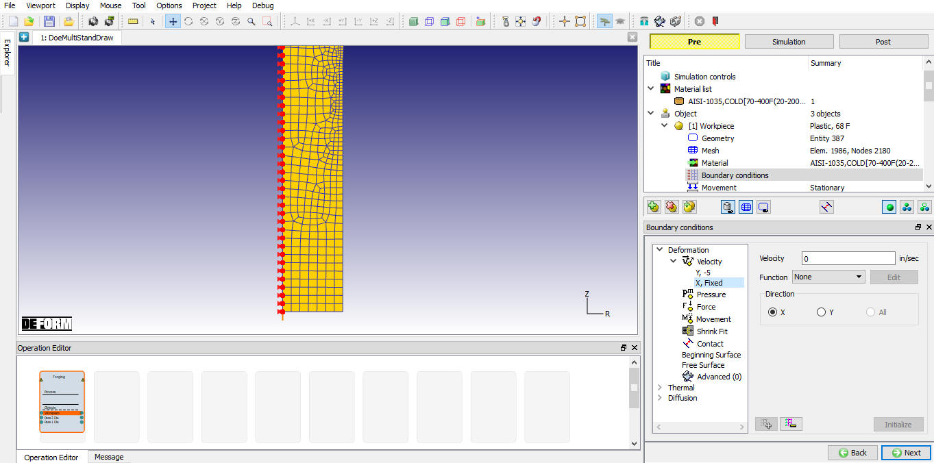
Imported keyfile is an Multi stand drawing setup having 2 stands, each stand dies are named as pass1 Die and Pass2 Die. Workpiece is pulled in these dies to perform the drawing process, this is accomplished by applying velocity for Workpiece.

Select the Workpiece Boundary Conditions from operation tree to observe the workpiece velocity Boundary Conditions defined at the front end to pull the workpiece through the dies and fixed velocity at the centerline as shown in Fig. DOEL1.5.

Workpiece front end velocity boundary condition

Similarly select the X Fixed velocity BCC and observe the centerline fixed velocity as shown in Fig. DOEL1.6.

Workpiece centerline velocity boundary condition

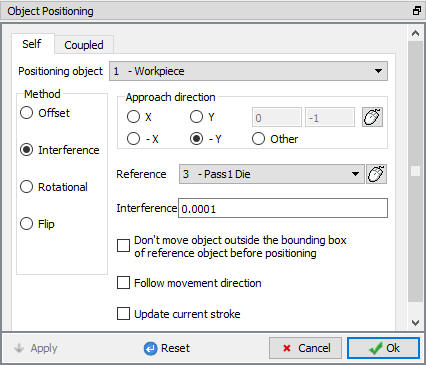
As we vary the Pass1 Die diameter in DOE project, Workpiece has to position with respect to varied die geometry diameter by interference in –Y direction during DOE simulations. So we have to schedule workpiece position with respect to die.

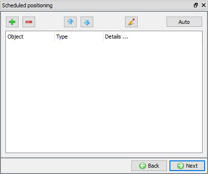
Click on Scheduled position in operation tree to define the scheduled positioning of workpiece with respect to Pass1 Die. Click on (Add) button to add the scheduled positioning definition (See Fig. DOEL1.7.) and interference position the Workpiece with respect to Pass1 Die in –Y direction a shown in Fig. DOEL1.8.

Scheduled positioning window

Interference positioning Workpiece with respect to Pass1 Die

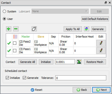
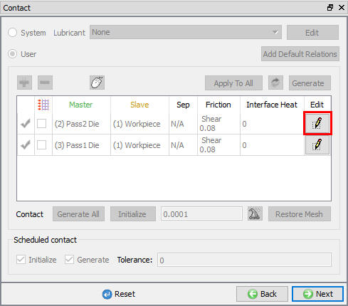
Click to close the Scheduled positioning definition. Select Contact in operation tree to observe the Inter-object relationship between Dies and Workpiece and its friction coefficient value. (See Fig. DOEL1.9.)

Inter-object relationship window

Select the Generate Database in operation tree, when we visit Generate Database we will get “Apply scheduled Positioning “ popup due to scheduled positioning data, click “Yes “ in popup and generate Database. (See Fig. DOEL1.10.)

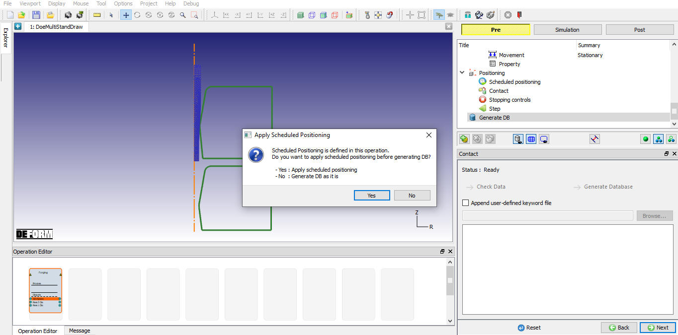
Generate database window

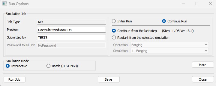
Click on MO Mode button to submit to simulate. Click on the action label to open the Run Options dialog as shown in Fig. DOEL1.11. Use the default Continue Run option to select “Continue from the last step ”option and then select the Simulation mode as Interactive and click on button to run the simulation.

Run simulation window

After completing the simulation click on MO mode button to play the steps and check the nominal simulation as shown in Fig. DOEL1.12.

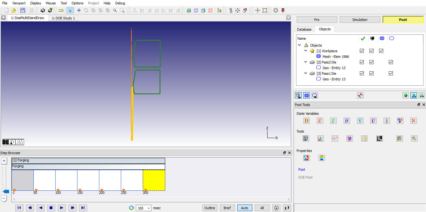
DOE nominal project post mode

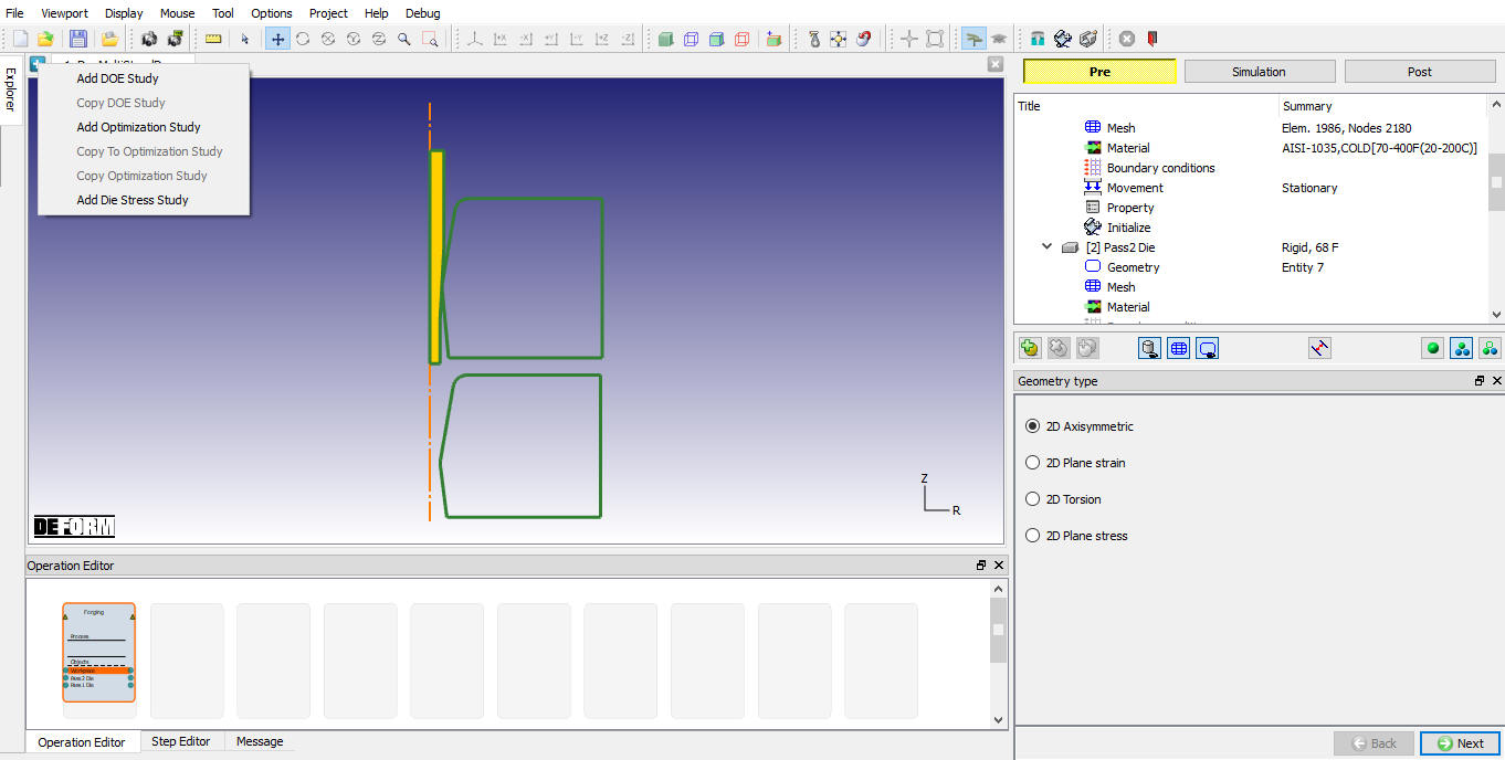
Add DOE Project

Click on MO mode button to add the DOE Study. Click on (Add) button at top left corner of graphics window and select Add DOE Study option as shown in Fig. DOEL1.13.

Adding DOE Study Project

DOE project will be added along with the DOE output operation needed to study the DOE results as shown in Fig. DOEL1.14.

Added DOE Study Project

Add die geometry variation as DOE variable

Select the Forming operation from Operation Editor to add DOE variables. To vary the first stand die diameter select Pass1 Die Geometry from operation tree and add geometry as DOE variable by clicking on (Add DOE Variable) button as shown in Fig. DOEL1.15.

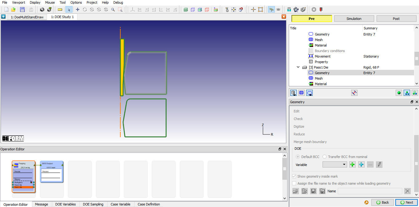
Adding geometry as DOE variable

Name the DOE variable as “Dia” and select the number of samples as 2. User can add the Description about the DOE variable definition, in this lab as we varying internal dia from 0.2 to 0.24 add the description as “Internaldia is varied from 0.2183 to 0.2 for lower bound and 0.24 for upper bound. ” as shown in Fig. DOEL1.16.

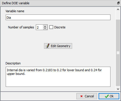
DOE variable definition window

Click on to define lower and upper bound geometry. In 2D geometry editor confirm that the DOE type is Lower. (See Fig. DOEL1.17.)

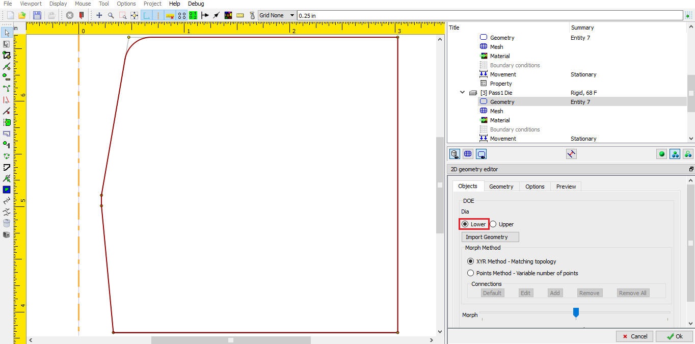
2D DOE geometry editor window

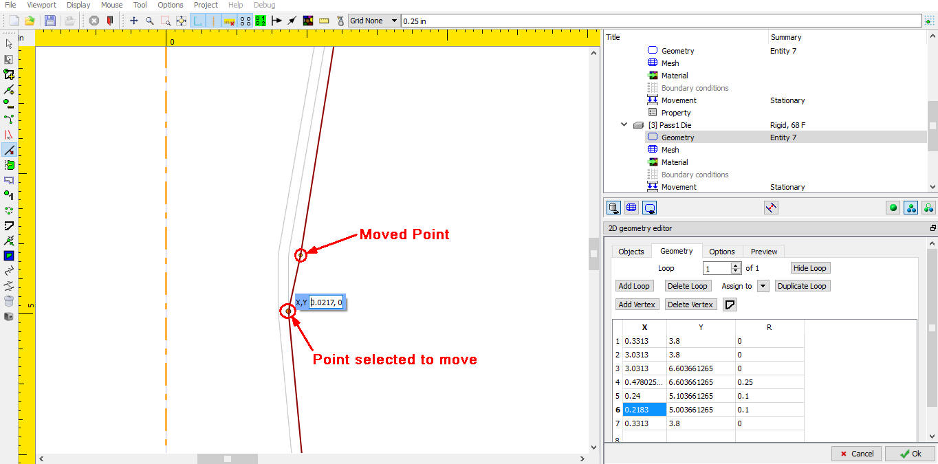
Click on Geometry tab to observe the internal flat region dia 0.2183 in X column of the table. Select the innermost dia point and select the (Move) icon and move the point by (-0.0183,0) as shown in Fig. DOEL1.18.

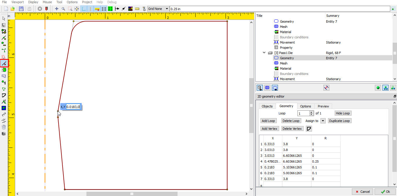
Moving the internal dia points for lower bound geometry

Similarly move other end of the flat dia point 0.0183 in towards centerline as shown in Fig. DOEL1.19.

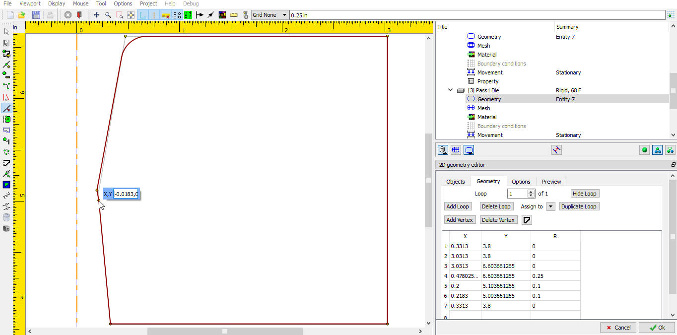
Moving 2nd dia flat point

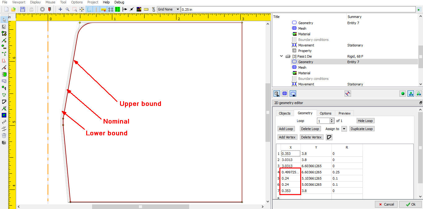
In order to maintain the same entry and exit angle of the die, move the top and bottom taper edge end points for the same amount towards centerline. Finally the lower bound geometry and geometry table looks as shown in Fig. DOEL1.20.

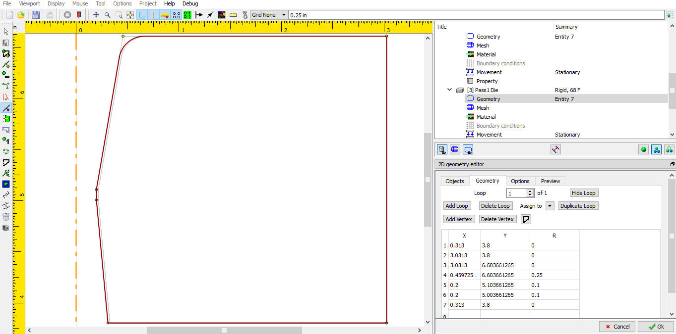
Lower bound geometry

Select objects tab to define the upper bound of DOE geometry variable and select the Upper for DOE type as shown in Fig. DOEL1.21.

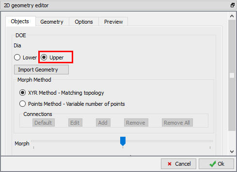
Upper bound geometry variable selection

Select back the geometry tab and move the internal flat dia points by 0.0217 away from centerline, so the dia changes from 0.2183 to 0.24 as shown in Fig. DOEL1.22.

Moving Upper bound internal flat dia points

Similar to the flat edge end points move the top and bottom taper edge end points for the same amount away from centerline in order to maintain the same entry and exit angle of the die. Finally the upper bound geometry and geometry table looks as shown in Fig. DOEL1.23.

Upper bound final geometry points

Click on objects tab and drag the morph sliding bar to observe the transition of the geometry variation from lower to upper bound as shown in Fig. DOEL1.24.

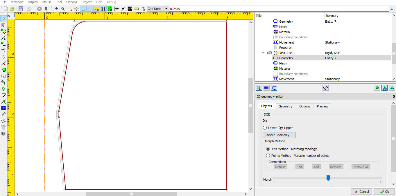
Morphed geometry between defined geometry variations

Click to close 2D Geometry Editor and again click to close the Geometry DOE variable definition for Pass1 die. Observe the green color fill around the (edit geometry) button (See Fig. DOEL1.25.) indicating the DOE variable defined successfully. If the definition having any errors then red color fill can be observed around the DOE variables field.

Geometry window after DOE variable definition

Add Friction coefficient as DOE variable

Select the Contact in operation tree to define the Pass2 die and workpiece friction coefficient as second DOE variable. (See Fig. DOEL1.26.)

Inter object definition window

Click on for Pass2 Die and Workpiece contact relation (See Fig. DOEL1.26.). Right click on the constant Friction field and add as DOE variable as shown in Fig. DOEL1.27.

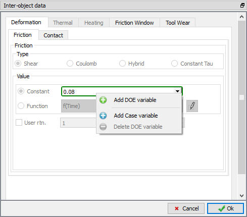
Inter object relations edit window deformation tab

DOE variable definition window will open (See Fig. DOEL1.28.). Name the DOE variable as “Friction “, number of samples as 2, define upper value as 0.084 and lower value as 0.076 as shown in Fig. DOEL1.28. For this variable we add the description as “Friction coefficient varied 5 percentage above and below the nominal value. “.

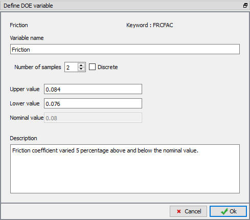
DOE variable Friction coefficient definition window

Confirm the DOE variable definition not having any error by green color fill around the friction coefficient value field as shown in Fig. DOEL1.29.

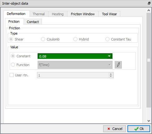
Inter object edit window deformation tab after DOE variable definition

Click to close Edit Inter-Object definition window.

Check DOE Variables table

Select the DOE Variables table to observe the defined DOE variables list (See Fig. DOEL1.30.). User can edit the DOE variable definition easily from the DOE Variables table for constant values by double click on the values. Function values can be edited by clicking on the single Edit button below the Upper value column.

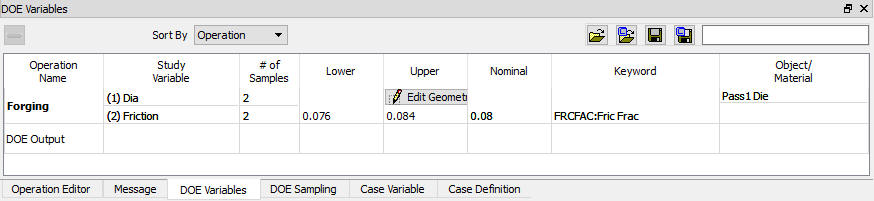
DOE variables list in DOE variables window

DOE Samples definition

Select the DOE Sampling tab and select sampling method as Full Factorial and observe the total number of simulation text next to it as shown in Fig. DOEL1.31. In this lab as the number of samples for both the DOE variables are 2, total number of DOE Runs/Simulations becomes 4 (2x2).

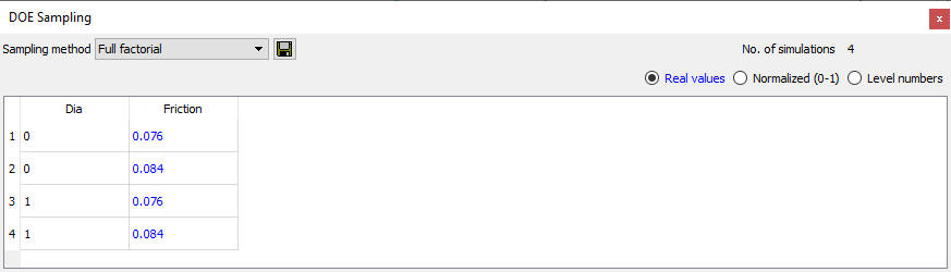
DOE Sampling window

Define DOE Output operation

Select DOE Operation and object to Study

Select DOE output operation from operation editor and select the forming operation check box in operation selection window (See Fig. DOEL1.32.). If the Nominal project is having more than one operation and DOE variables are defined more than one operation then user can select the both the operations to study. Click to define the Output types.

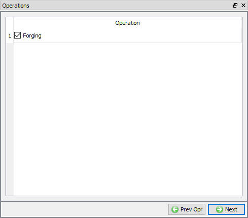
Operation Selection window

Define Output variables

Check the Operation min/max value, Local min/max value and SV on all nodes/elements (Last step of selected operation) output types (see Fig. DOEL1.33.). Click to define the Region of Interest.

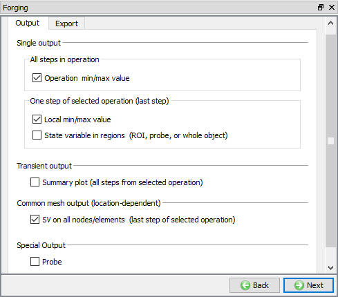
DOE Output selection window

Click on (Add) button to add region and click on (See Fig. DOEL1.34.).

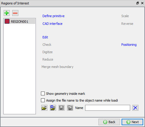
Region of interest window

Create the hollowcylinder primitive of Radius 1.1 and Height 1.5 (See Fig. DOEL1.35..). Click to close the geometry definition. Click on P**osi tioning and define **Offset as (-0.1, -1) as shown in Fig. DOEL1.36. and then click on .

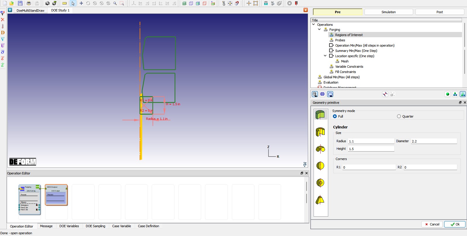
Region of interest geometry creation

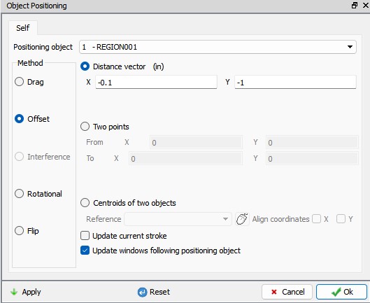
Positioning of Region of Interest

Click to Operation Min/Max (All steps in operation) and add Effective Stress and Effective Strain state variables as shown in Fig. DOEL1.37. Minimum value as component, select Max in Min/max and workpiece as Object and click .

Operation Min/Max output variables definition window

Click twice to add Minimum Effective Stress and Strain at last step of the operation as summary variables and Workpiece as Object as shown in Fig. DOEL1.38.

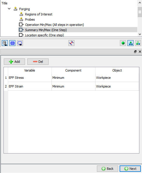
Summary Min/Max variables definition window

Click and click button thrice to define 3 Location specific state variables. Add Effective Strain , Effective Stress and Effective Strain rate state variables and select the Common Mesh Region as REGION001 at the bottom of the window as shown in Fig. DOEL1.39.

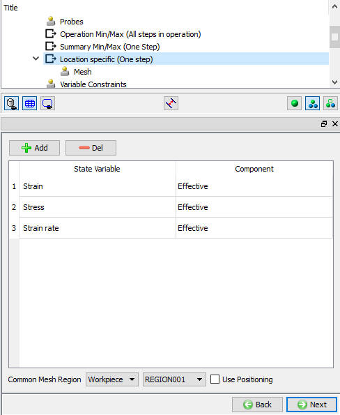
Location specific (all nodes) variables definition window

Selecting the defined Region of Interest region as Common Mesh Region system adds the Mesh window next to this. So click and click on button to generate mesh for the region as shown in Fig. DOEL1.40.

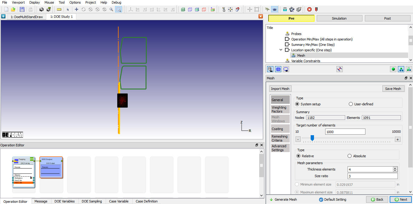
Region of interest region mesh generation window

As we are not defining any Variable and Fill constraints click on (Save project) icon. If user want to limit any state variable value user can define variable constraints or if user need to filter the underfill and lap deflects user can check fill constrains.

Select MO mode button to submit DOE project to simulate.

Simulate DOE project

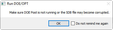
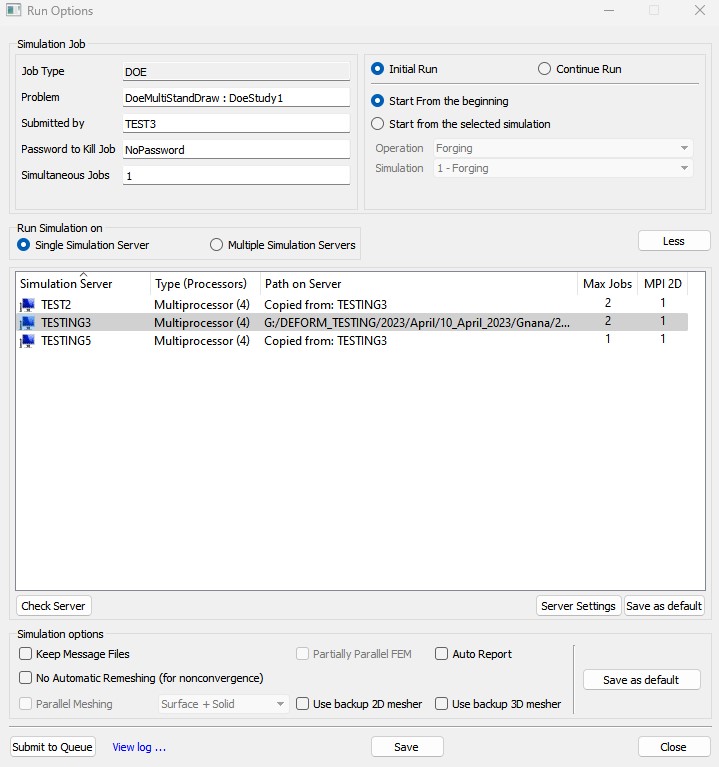
Click on button to submit to simulate Click for Run DOE/OPT pop-up (See Fig. DOEL1.41.) and select the simulation server in the available Sim Server list. Click on button (See Fig. DOEL1.42.) to start DOE samples DB generation and simulations. System generates the database for all runs and then start simulating from DOE Run 1 to Run N (last Run) in queue. If user selected more than one Simultaneous simulations then selected number of simulations will run simultaneously.

DOE simulations Run window

Observe the Simulation Jobs tab to monitor the DOE running jobs status as shown in Fig. DOEL1.43.

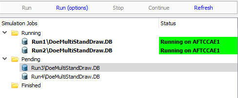
DOE runs Simulation jobs status

Select the DOE Log file to observe the DOE running jobs more details as shown in Fig. DOEL1.44.

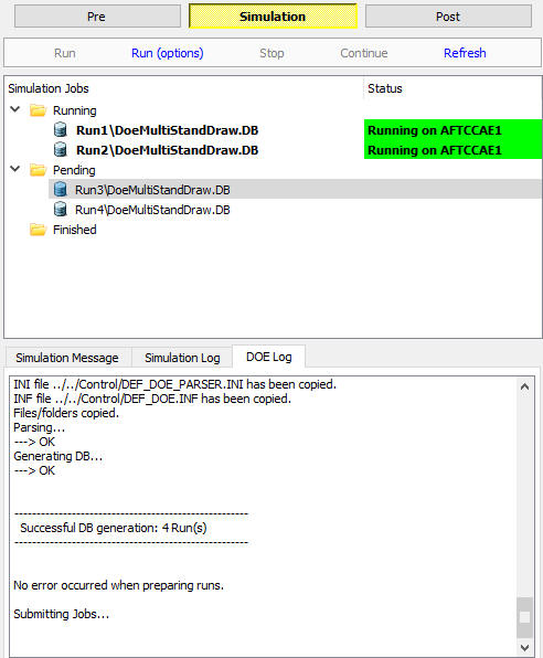
DOE jobs Log details

From DEFORM Main GUI explorer window user can observe the file structure for the DOE projects as shown in Fig. DOEL1.45.

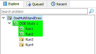
DOE Project file structure

Confirm the DOE runs simulation by ‘Simulation is done” message in DOE Log tab then click on MO mode button to open the DOE post.

Review the DOE results

In MO Post click on button to open the DOE SQL Database file (SDB) in DOE post as MO Post do not give the DOE results statistical analysis features. DOE Post will open in other window as shown in Fig. DOEL1.46.

DOE Post

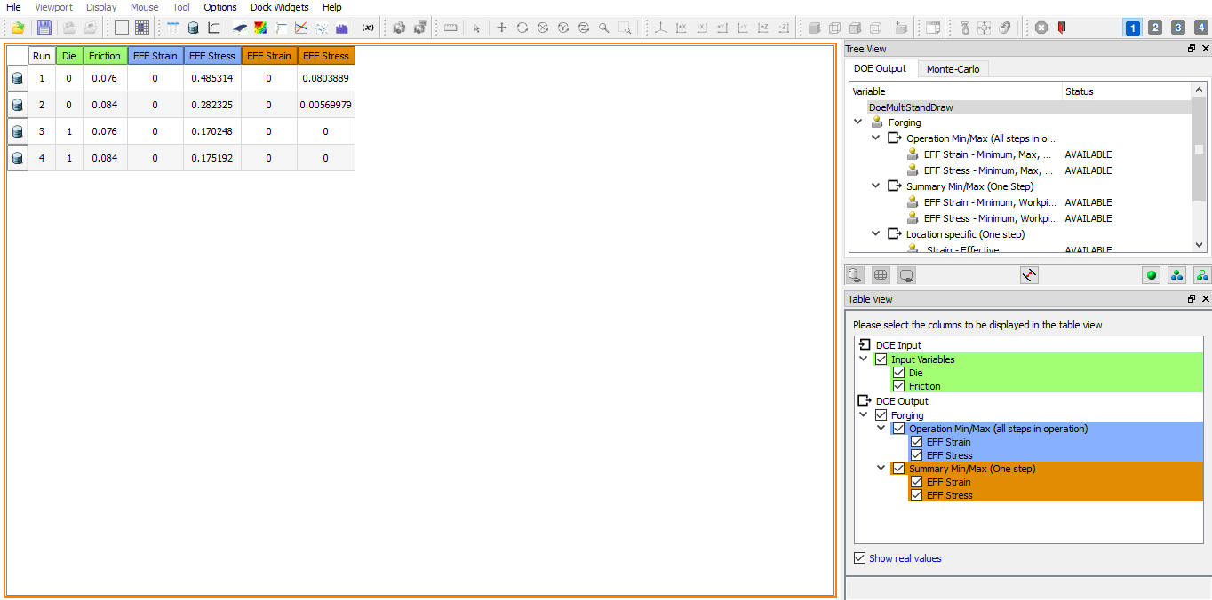
Table view will be displaying in the graphics window. We can select respective check boxes in the property window area which to be displayed in the table view (DOE Input and DOE Output).

Check Operation min/max (all steps) variables

Select the Operation Min/Max variable in output tree and click on table view. All DOE runs global minimum values are zero, so no need to plot other curves.

In table view for Diameter DOE geometry variable Dia 0 indicates lower bound geometry and 1 indicates upper bound geometry, as we are taken only 2 samples there is no geometry variation between lower and upper bound. In such case it display fraction value, if it is more than 0.5 it indicates between nominal and upper bound.

Check Summary min/max (last step) variables

Select Summary Effective Strain and click on (3D response surface plot) icon to observe the 3d representation of this response for input DOE variables. (See Fig. DOEL1.47.).

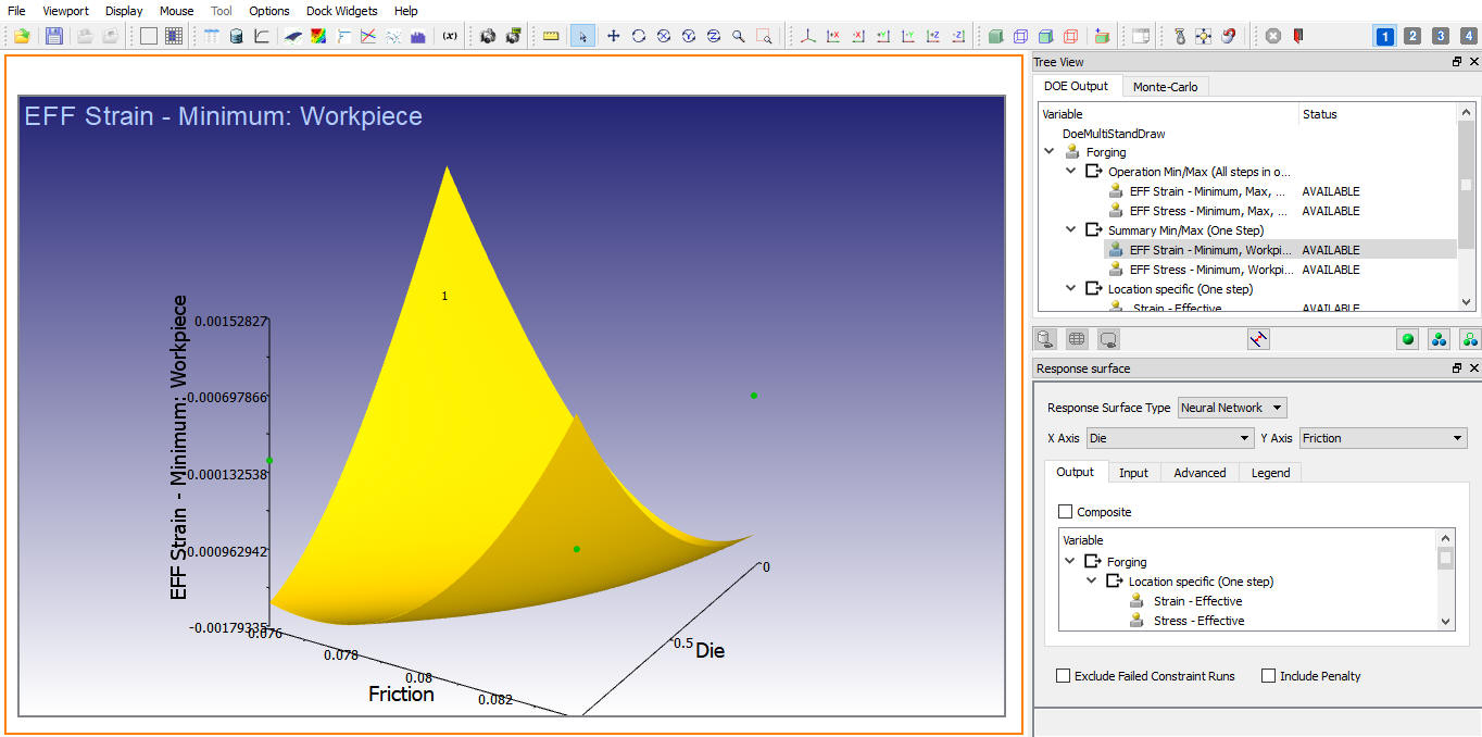
Minimum Effective Strain summary response surface

Click on (2d contour response surface) to view the response of selected output variables on 2d plane as shown in Fig. DOEL1.48. From tool menu bar select Change layout button and select “Grid4_1” to divide graphics area equally for all 4 windows as shown in the Fig. DOEL1.48.

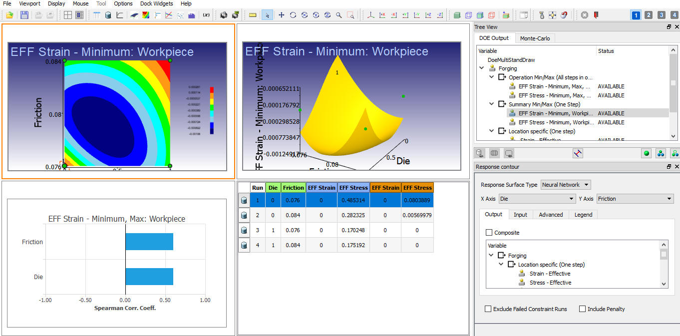
2D contour response surface for Minimum Effective stress

Also, try-out the tornado, sensitivity, scatter and histogram plots to analyze the Minimum Effective stress output variable. (See Fig. DOEL1.49.)

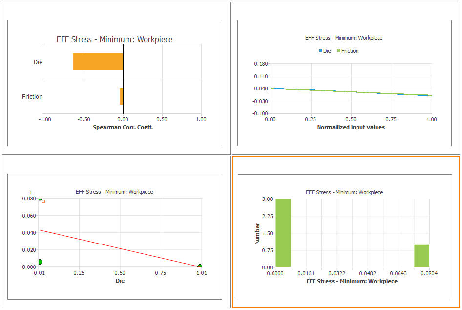
DOE variables sensitivity plots for Minimum effective stress summary variable

Tornado chart gives relative magnitude and direction of influence of DOE variables selected output variable. In the Fig. DOEL1.49. tornado chart indicating Diameter is having more influence compared to Friction on Minimum effective stress at last step and both are inversely affecting.

Sensitivity plot show the effect of each DOE study input variable to the selected output variable as slope. For Minimum effective stress both input variations are inversely affecting.

Scatter plot show correlation between DOE study input variable and selected output variable by linear regression. In the above Fig. DOEL1.49. we can observe the linear regression equation along with the sampling points.

Histogram plot shows the frequency of the DOE runs output variables within small ranges. So it’s an Number of DOE runs Vs Selected output variable bar graph.

Check Location specific (One step) variables

Select the location specific Effective strain value in the DOE Output tree. As explained in the Summary variables check plot the 3d and 2d response surfaces and observe the output variable response for the selected input as shown in Fig. DOEL1.50. For location specific output variable it will plot the state variable information only for the defined region of interest when we are in the common mesh tab as shown in Fig. DOEL1.50.

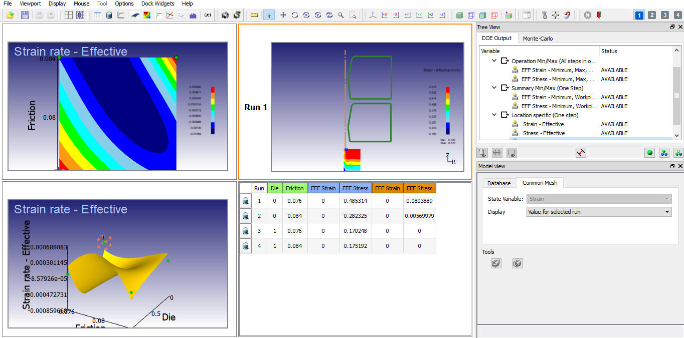
3D and 2D Response surface plot for location specific Effective strain

For more details on these post analysis features refer the chapter 54. DOE Post Processor.

52.2. DOE Simulation Running and Monitoring

54.1. DOE Post Processor