Lab 3. Spike Forging
3.1. Spike Forging - Transfer from Furnace to Dies
3.2. Spike Forging - Dwell On Bottom Die
3.3. Spike Forging - Forging Blow1
3.4. Spike Forging - Die Change and Blow2
In four operations, a hot spike forging will be modeled. Since the process is hot, the most accurate simulation will model not only the forging operation but also any heat transfer operations that occur. The entire process will be divided as follows:
-
Heat transfer operation will model a 10 second transfer of the billet from the furnace to the dies. This is solely a heat transfer simulation.
-
Dwelling Operation will model the 2 second dwell period of the billet resting on the bottom die prior to forging. This is also a heat transfer simulation.
-
Forming operation will model the first blow and do a Die change for Second Blow of a two blow forging process.
To perform Die Stress for this setup, please refer to Die Stress Wizard lab 2.
Since the billet and dies are axisymmetric, the process could be modeled in 2D. However, in order to further explore symmetry and other important 3D concepts, the process will be modeled in 3D using 1/4 symmetry for the billet and the dies.
Spike Forging - Transfer from Furnace to Dies
Create a new problem either by selecting File ![]() New Problem or by clicking the New Problem
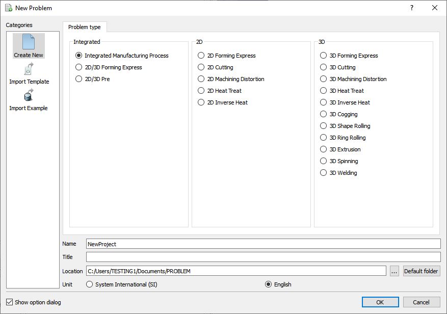
New Problem or by clicking the New Problem ![]() icon. The Problem Setup window will appear as shown in Fig. 3DL3.1. Select “Integrated Manufacturing Process “ radio button and unit system as “English “ radio button in unit field. Define Problem Name as “Spike_Forging “ and make sure the “Show option dialog ” check box is turned on (if we do not turn on the “Show option dialog” check box, then we will not get the New Project dialog). Then click on
icon. The Problem Setup window will appear as shown in Fig. 3DL3.1. Select “Integrated Manufacturing Process “ radio button and unit system as “English “ radio button in unit field. Define Problem Name as “Spike_Forging “ and make sure the “Show option dialog ” check box is turned on (if we do not turn on the “Show option dialog” check box, then we will not get the New Project dialog). Then click on ![]() button to open a new problem using the Deform Integrated Manufacturing Process.
button to open a new problem using the Deform Integrated Manufacturing Process.
MO wizard will open at this point user will be prompted to specify a project name (system will create a separate folder with this project name) and title for this session. In this session we use ‘Spike_Forging ’ as the project name. User can also change the Unit system (File menu selected unit system will be selected by default) and add operation by selecting from First operation pull down list and checkbox. Using copy Existing project option we can import previous saved projects as new project. Click on ![]() to continue to open the operation.
to continue to open the operation.
Assigning problem name
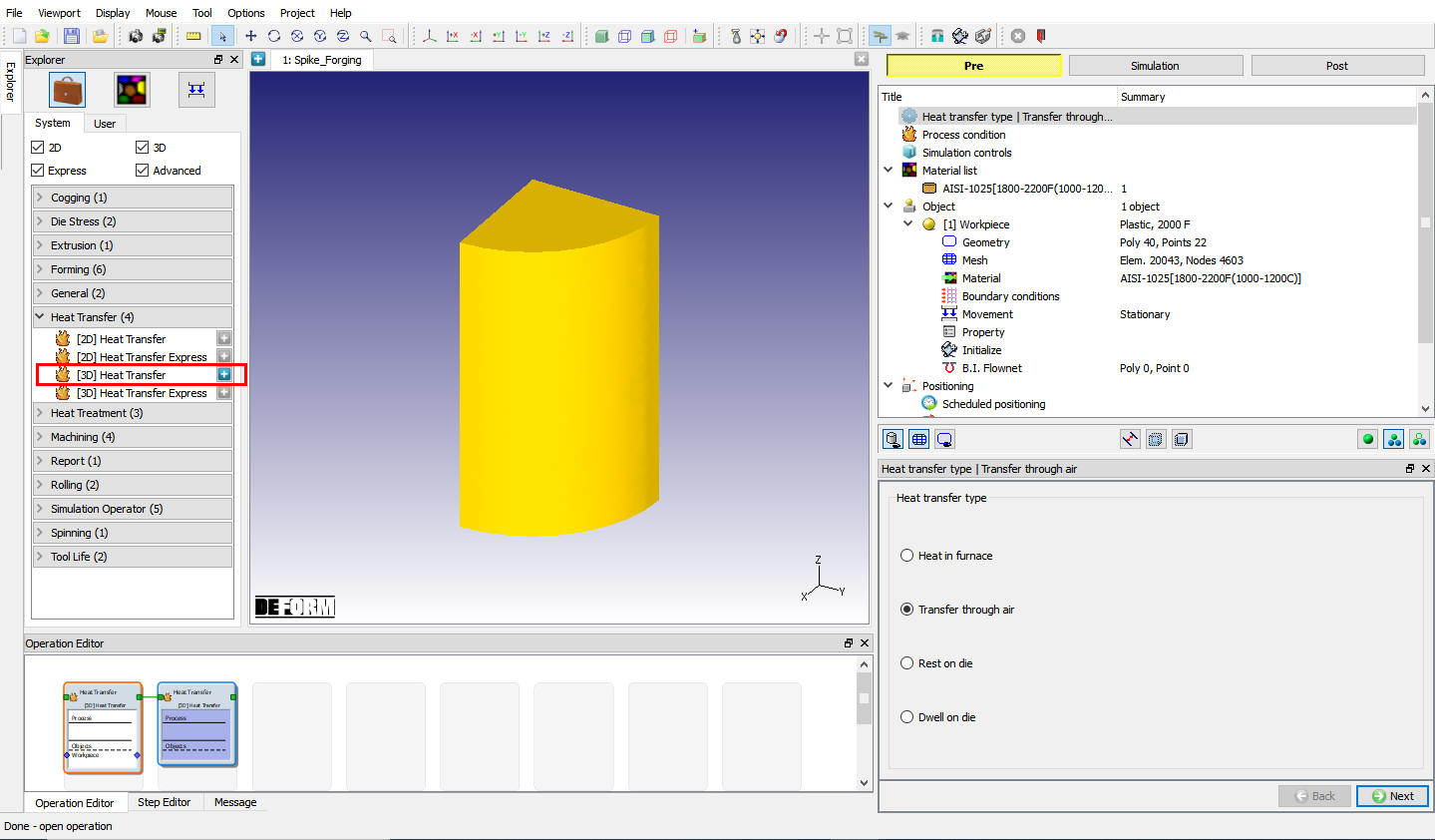
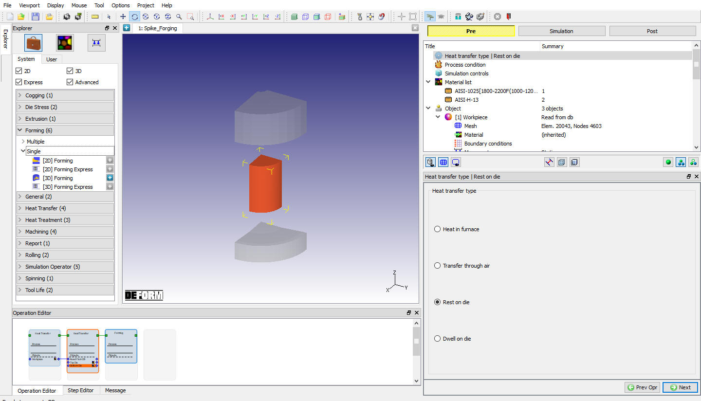
Multiple Operation wizard will open. Add 3D Heat Transfer operation from the Explorer Operations list. Add the operation by clicking on ![]() button next to 3D Heat Transfer or user can also add by drag and drop into the Operation Editor. (See Fig. 3DL3.2.)
button next to 3D Heat Transfer or user can also add by drag and drop into the Operation Editor. (See Fig. 3DL3.2.)
MO Wizard Window
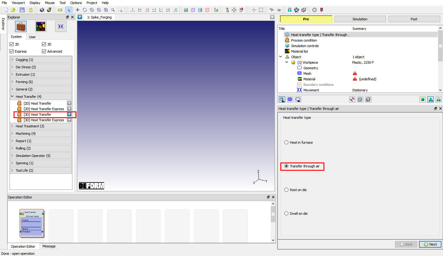
Assign Heat transfer Type
Since we are doing Air transfer operation, select the Heat transfer type as Transfer through Air. click ![]() .
.
Assign Process Condition
Define heattransfertime as 10 sec and keep rest other fields as it is. (See Fig. 3DL3.3.) . Click ![]() until Object page.
until Object page.
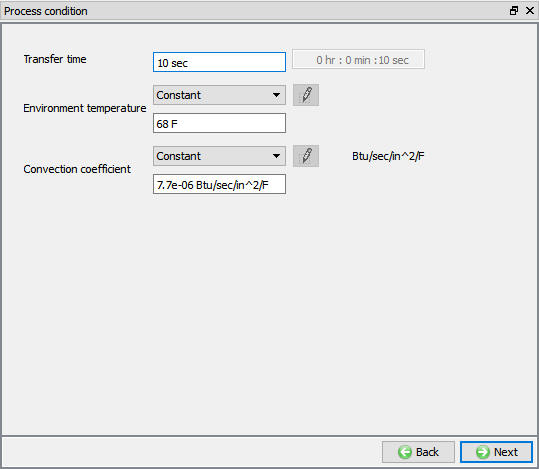
Assigning Transfer operation Process condition
Objects
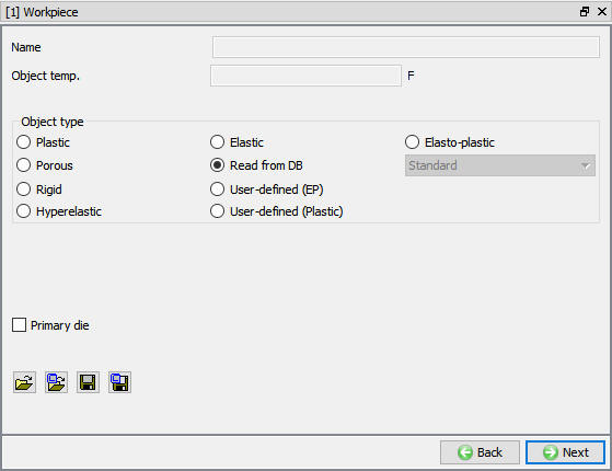
In this initial heat transfer simulation, the billet will be getting transferred from the furnace to the dies. For this operation by default only one object will be added in list, use the default selection and (see Fig. 3DL3.4.) click on ![]() .
.
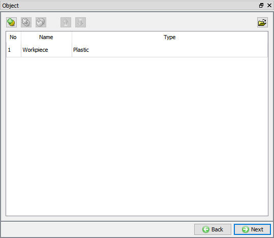
Objects window
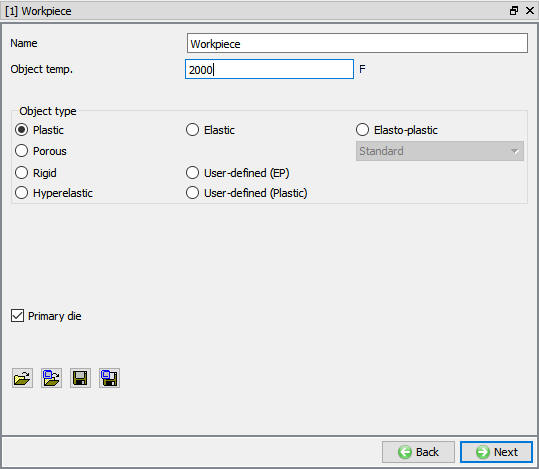
Defining Object Temperature
In Workpiece page Define Object temperature as 2000 °F as shown in Fig. 3DL3.5. Click on![]() .
.
Defining Workpiece temperature
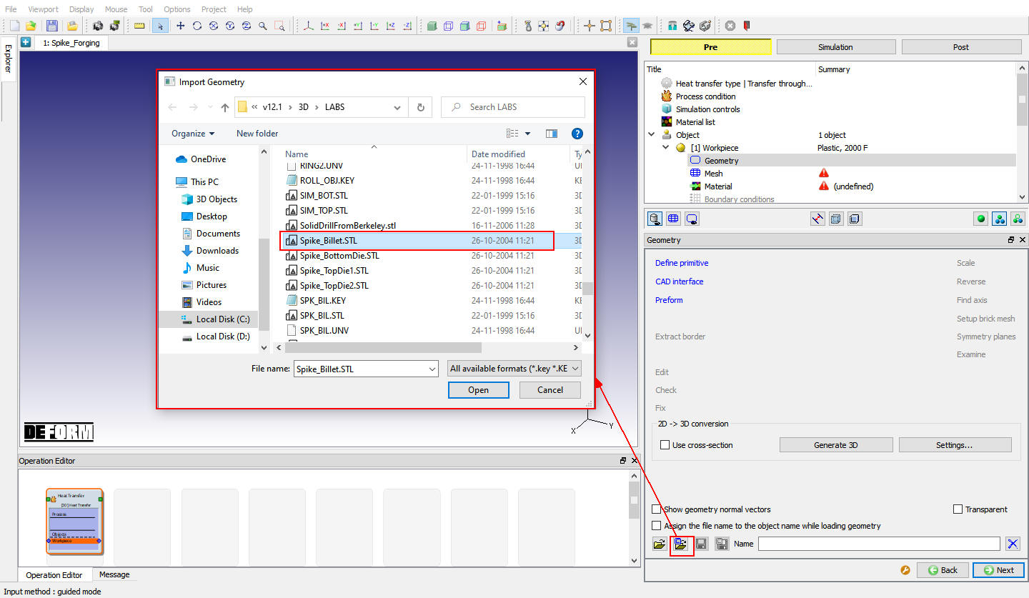
Import Geometry
In Geometry page, click on import geometry from library option (![]() ) and import the Spike_Billet.STL file from DEFORM installed folder \3d\LABS directory as shown in Fig. 3DL3.6. Use
) and import the Spike_Billet.STL file from DEFORM installed folder \3d\LABS directory as shown in Fig. 3DL3.6. Use ![]() action label to check the Geometry. A perfect geometry should display message as shown in Fig. 3DL3.7.
action label to check the Geometry. A perfect geometry should display message as shown in Fig. 3DL3.7.
Importing Geometry
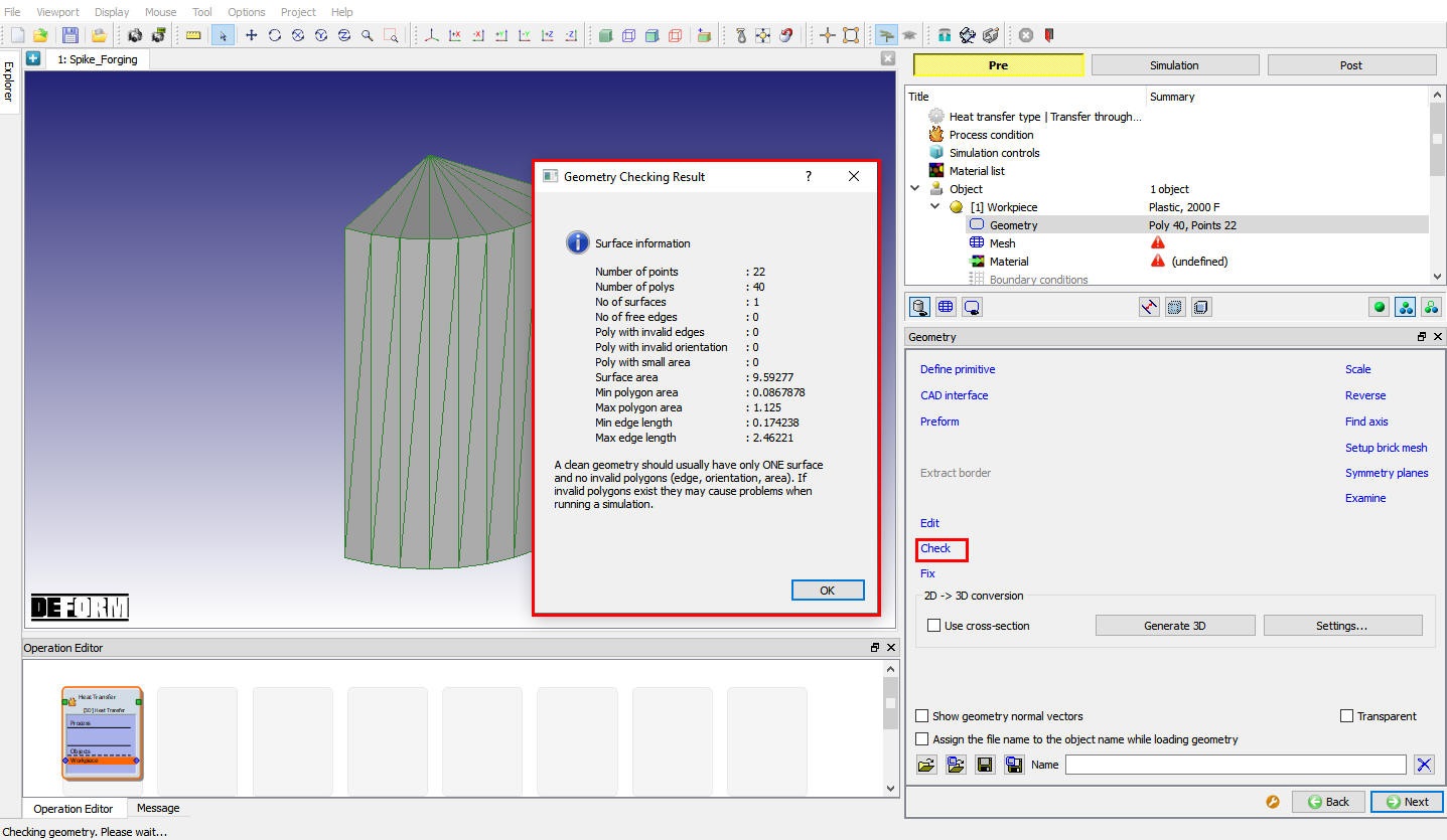
Geometry Checking popup
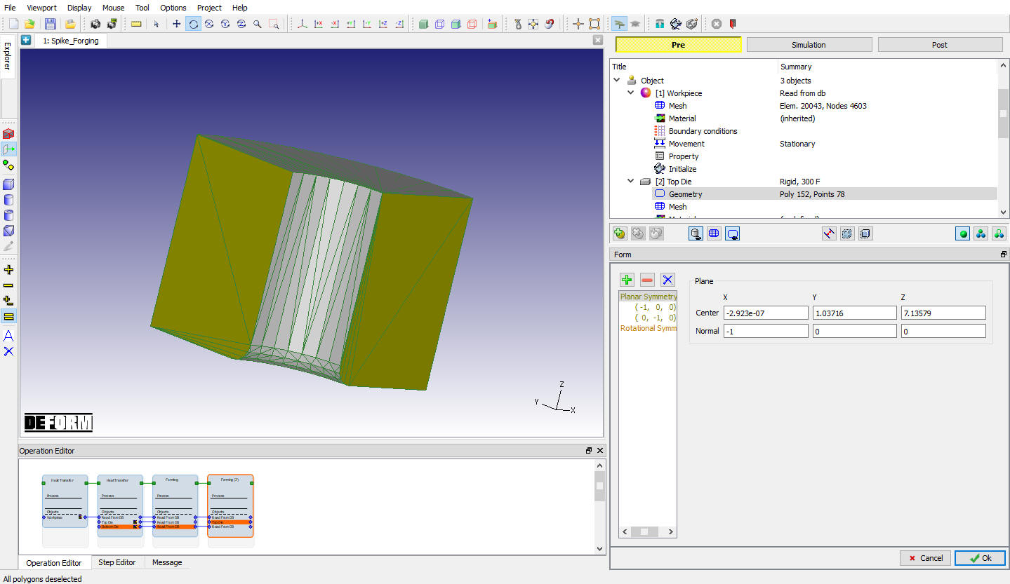
Assigning Symmetry Conditions
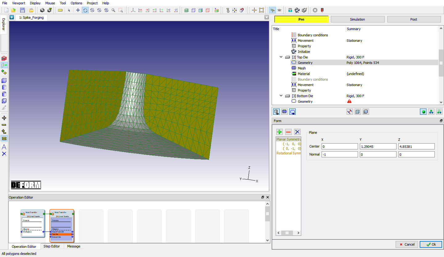
Click on the ![]() option, select one of the symmetry planes of the Workpiece and click the to define planar symmetry as shown in Fig. 3DL3.8. Repeat this for the other symmetry plane then click
option, select one of the symmetry planes of the Workpiece and click the to define planar symmetry as shown in Fig. 3DL3.8. Repeat this for the other symmetry plane then click ![]() . Click on
. Click on ![]() .
.
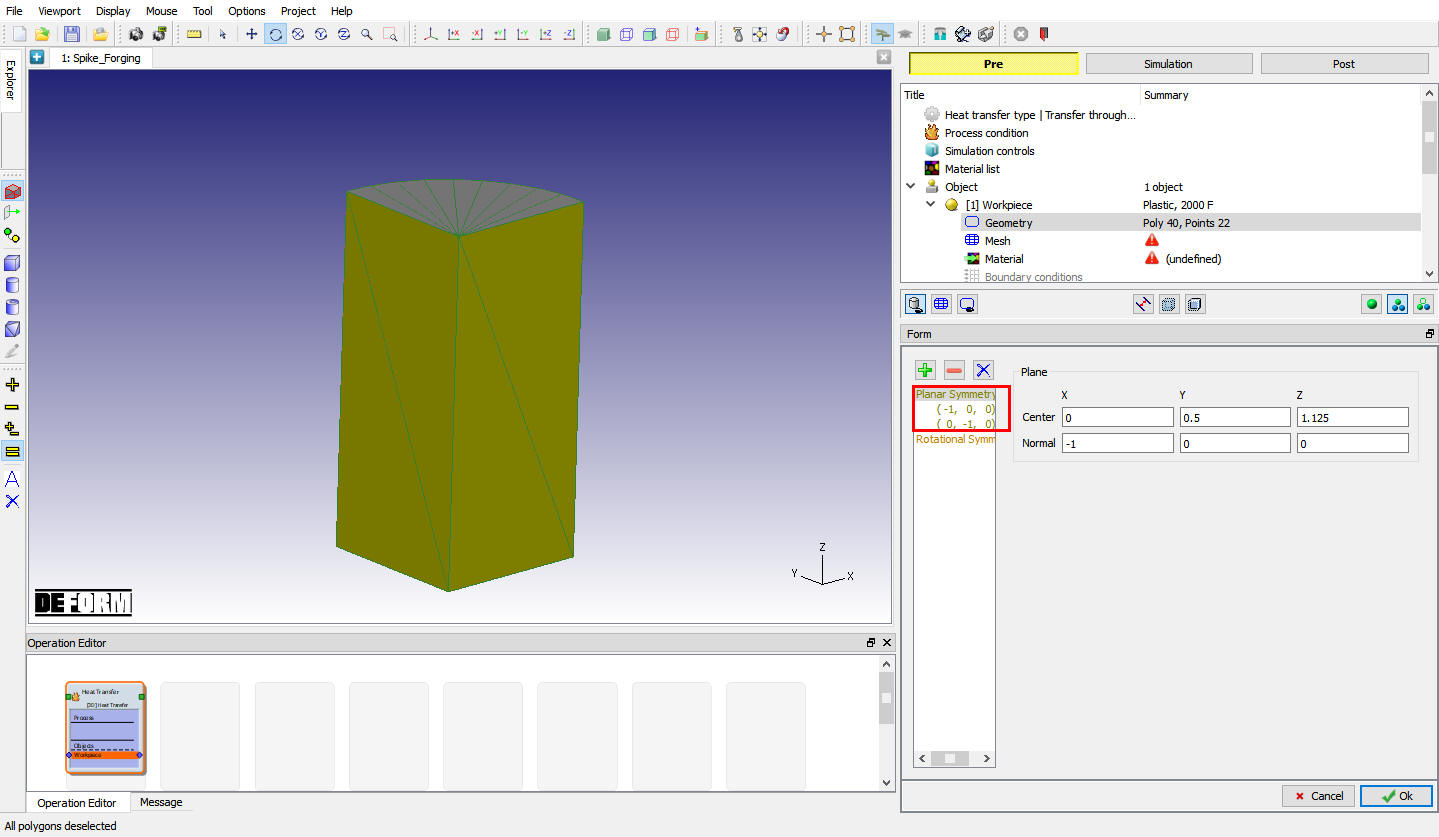
Assigning Planar symmetry to the workpiece
Meshing the Workpiece
Switch to Expert mode by clicking on ![]() (Switch to expert mode) icon from the tool bar. Expert mode will provide more options for detailed settings.
(Switch to expert mode) icon from the tool bar. Expert mode will provide more options for detailed settings.
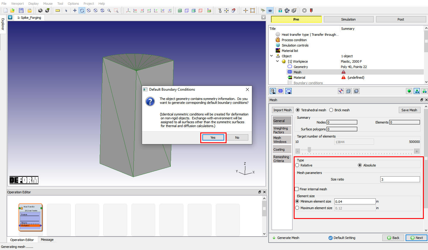
In Mesh page, Select Absolute type, set the Min Element Size to 0.04 and also set the SizeRatio to 3. After changing these settings, click on ![]() . Click
. Click ![]() for Default Boundary condition popup. (See Fig. 3DL3.9.) Click on
for Default Boundary condition popup. (See Fig. 3DL3.9.) Click on ![]() .
.
Defining Mesh Data
Assigning Material to the Workpiece
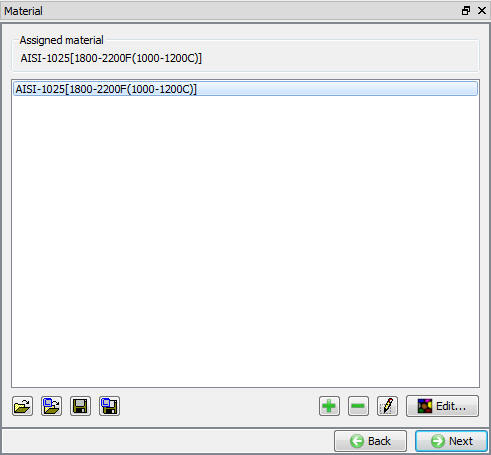
In Material Window, click on to Load material data from Library ![]() and load ‘AISI-1025[1800-2200F(1000-1200C)] ‘ material from Steel category by clicking
and load ‘AISI-1025[1800-2200F(1000-1200C)] ‘ material from Steel category by clicking ![]() button as shown in Fig. 3DL3.10. Select the added material from window to assign it to the workpiece as shown in Fig. 3DL3.11. Click
button as shown in Fig. 3DL3.10. Select the added material from window to assign it to the workpiece as shown in Fig. 3DL3.11. Click ![]() .
.

Material Window
Assigning Material to workpiece
Boundary Conditions
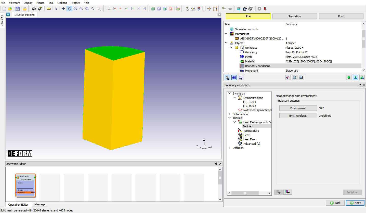
For this lab, Assigned Default Boundary conditions are OK for Workpiece in this setup (see Fig. 3DL3.12.). Click ![]() until Step page.
until Step page.
Boundary Conditions Window
Setting Step Controls
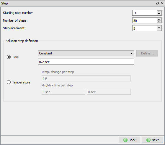
In Step Definition define Set the Number of Simulation Steps to 50 , the StepIncrement to Save at 5 and Solution step definition Time as 0.2 sec (see Fig. 3DL3.13.). Click ![]() .
.
Simulation Step Controls Window
Generate Database
By selecting the File menu ![]() Export option, save a keyword file for the problem as “Spike_Air_transfer “.
Export option, save a keyword file for the problem as “Spike_Air_transfer “.
Click on ![]() action label to check the problem. Generate database by clicking
action label to check the problem. Generate database by clicking ![]() action label.
action label.
Running Simulation
Once the database has been generated, switch to the Simulation mode by selecting the ![]() button above the object tree. Click on the
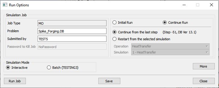
button above the object tree. Click on the ![]() action label under the simulation tab, Run Options dialog will open as shown in Fig. 3DL3.14.. Use the default Continue Run option to select “Continue from the last step ” option and then select the Simulation mode as Interactive and click on
action label under the simulation tab, Run Options dialog will open as shown in Fig. 3DL3.14.. Use the default Continue Run option to select “Continue from the last step ” option and then select the Simulation mode as Interactive and click on ![]() button to run the simulation.
button to run the simulation.
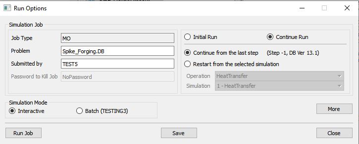
Run Simulation Window
Monitor the progress of the simulation by looking at the Simulation Message and Simulation Log tab, making sure that the ![]() option is checked. (See Fig. 3DL3.15.)
option is checked. (See Fig. 3DL3.15.)
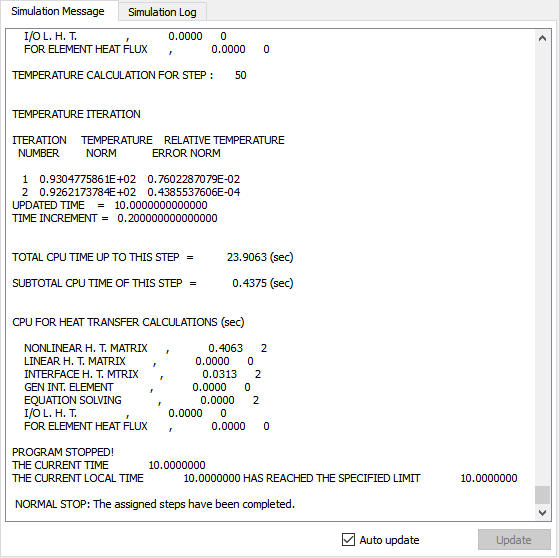
Simulation Message File
Post processing
When the simulation is complete, review the results by switching to Post mode using the ![]() button above the Simulation tool bar.
button above the Simulation tool bar.
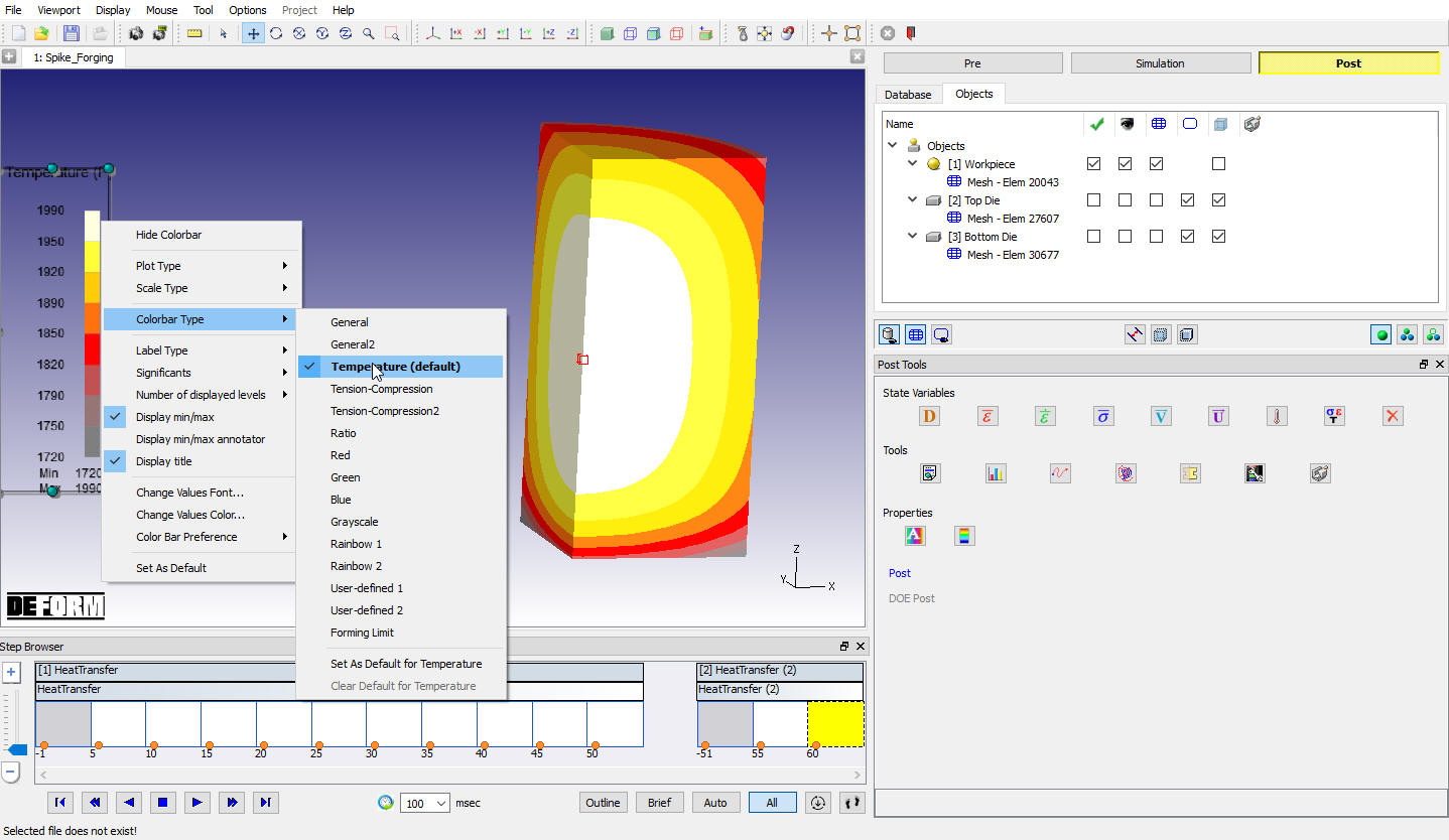
Plot Temperature State variable ![]() . Also, right-click on the Color Bar in the DISPLAY window and select Temperature as the Color Bar Type. This provides a more intuitive color scheme when viewing temperatures.
. Also, right-click on the Color Bar in the DISPLAY window and select Temperature as the Color Bar Type. This provides a more intuitive color scheme when viewing temperatures.
Play through the steps of the simulation and look at how the Billet cools down as it is transferred from the furnace to the dies. (See Fig. 3DL3.16.)
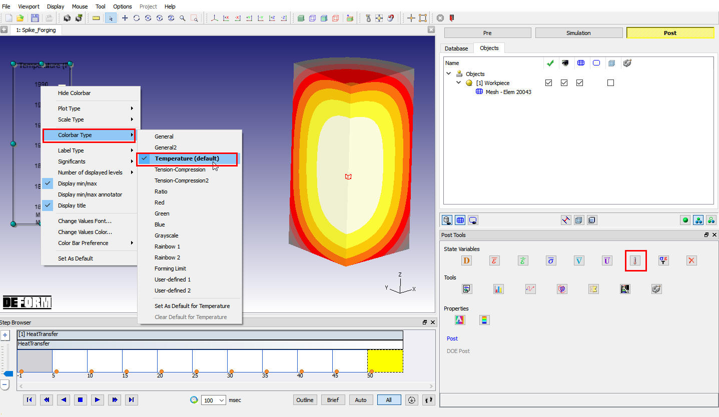
Post processor window with Temperature plot
Now, select last step in Step browser and click on ![]() button to continue the setup.
button to continue the setup.
Spike Forging - Dwell On Bottom Die
In earlier operation, workpiece was transferred from the furnace to the dies. Once the workpiece gets to the dies, it will rest on the bottom die for 2 seconds prior to forging operation. This dwell will be modeled in this operation. By selecting Batch mode setup type the dwell operation will be set up.
Add 3D Heat Transfer operation from the Explorer Operations list. Add the operation by clicking on ![]() button next to 3D Heat Transfer or can also be added by drag and drop into the Operation editor as shown in Fig. 3DL3.17.
button next to 3D Heat Transfer or can also be added by drag and drop into the Operation editor as shown in Fig. 3DL3.17.
MO wizard with two operations
Select 2nd operation from Operation editor, Setup type popup will appear and click on ![]() mode button (since we are setting up Dwell operation in Batch mode). See Fig. 3DL3.18.
mode button (since we are setting up Dwell operation in Batch mode). See Fig. 3DL3.18.
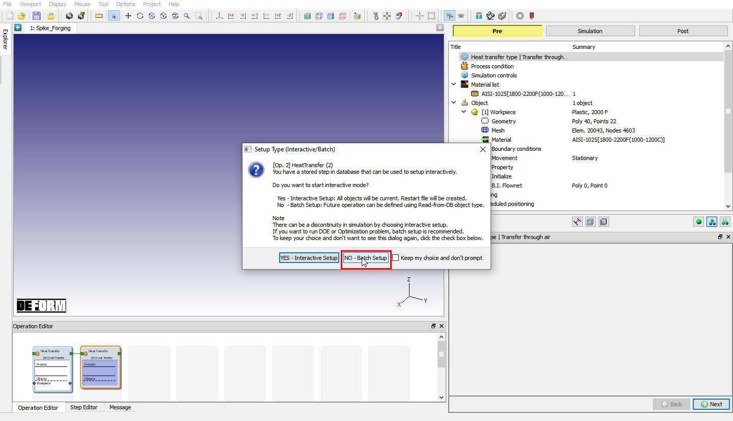
Setup type selection popup
In Heat transfer page, by default Rest on**Die **Heating type will be selected if not select Rest on Die Heat transfer type. Previous operation settings will be carried over the operation see Fig. 3DL3.19. Click on ![]() button.
button.
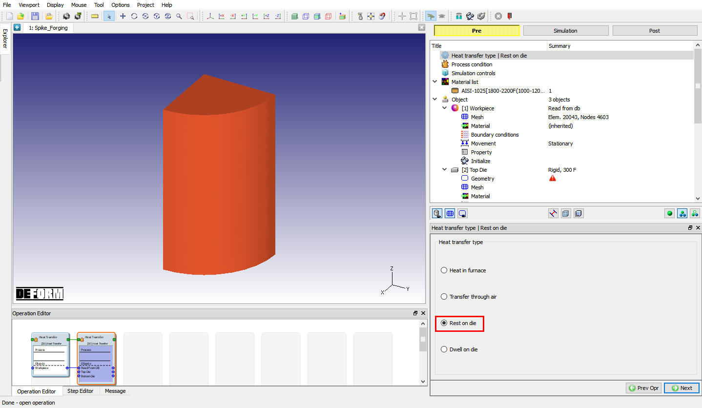
Heat Transfer type selection page
Process condition
Define RestingTime as 2 Sec, as the workpiece will rest on the bottom die for 2 seconds (See Fig. 3DL3.20.). Click ![]() until Objects page.
until Objects page.
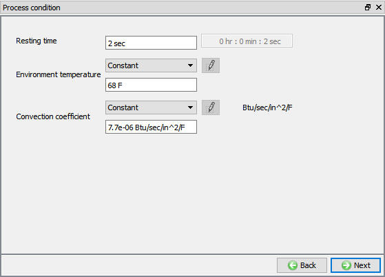
Resting operation Process Condition page
Adding Objects
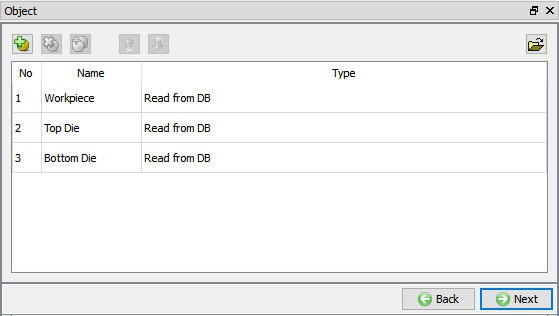
In Object page, by default 3 objects will be added. Depending upon the number of objects required for the simulation, user can add as many dies as needed by clicking on ![]() button. For this lab, we will use 3 objects (workpiece and 2 dies) (see Fig. 3DL3.21.). Click
button. For this lab, we will use 3 objects (workpiece and 2 dies) (see Fig. 3DL3.21.). Click ![]() .
.
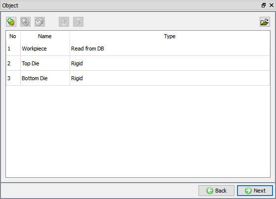
Objects window
Since we are continuing into heat dwelling operation from Heat transfer operation, Workpiece is automatically considered as read from DB object. As the object is read from DB type, all the data like temperature, mesh and BCC of the Object will be carried over from previous operation (see Fig. 3DL3.22.). Click ![]() until Top die page
until Top die page
Workpiece as Read From DB object
Top Die
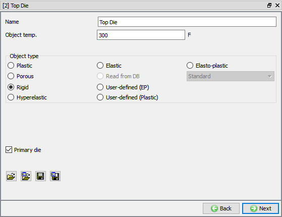
In, Top Die page, user can define required object temperature for Top die. For this lab default temperature 300°F is OK (see Fig. 3DL3.23.). Click ![]() .
.
Top die object window
Import Geometry
In Geometry page, click on import geometry from library option (![]() ) and import the Spike_Topdie1.STL file from DEFORM installed folder \3D\LABS directory. Use
) and import the Spike_Topdie1.STL file from DEFORM installed folder \3D\LABS directory. Use ![]() button to check the Geometry. Click on
button to check the Geometry. Click on ![]() option, define planar symmetry and click
option, define planar symmetry and click ![]() (see Fig. 3DL3.24.). Click
(see Fig. 3DL3.24.). Click ![]() .
.
Assigned Top Die plane Symmetry
Generate Mesh
Click on ![]() button and select yes in Default Boundary condition popup, a mesh with 28000 elements is generated.
button and select yes in Default Boundary condition popup, a mesh with 28000 elements is generated.
Assigning material Data
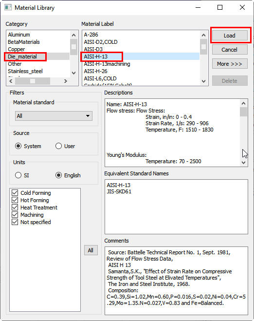
In Material Window, click on ![]() to Load material data from Library and load ‘AISI-H-13 ‘ material from Die_material category by clicking
to Load material data from Library and load ‘AISI-H-13 ‘ material from Die_material category by clicking ![]() button as shown in Fig. 3DL3.25. Select the added material from window to assign it to Top Die as shown in Fig. 3DL3.26. Click on
button as shown in Fig. 3DL3.25. Select the added material from window to assign it to Top Die as shown in Fig. 3DL3.26. Click on ![]() .
.
Material window
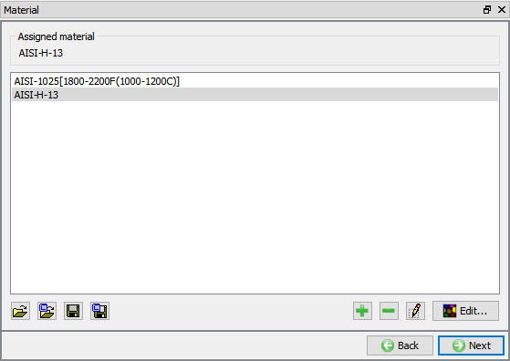
Assigning Material to Top Die
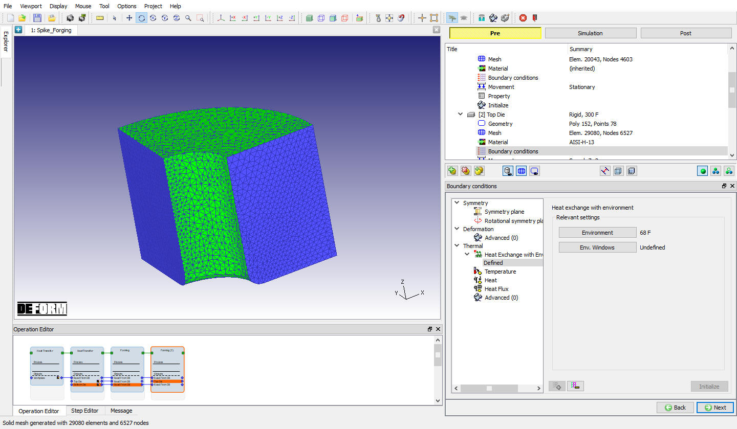
Assigning BCC
Assigned Default Heat Exchange with Environment Boundary conditions for Top die are OK ( see Fig. 3DL3.27.), click ![]() until Bottom Die page.
until Bottom Die page.
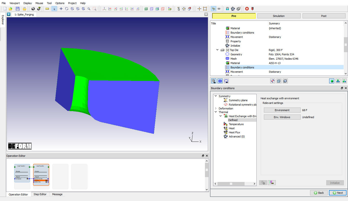
Assigned Heat exchange Boundary conditions for Top Die
Bottom Die
For this lab, default temperature 300°F is OK for Bottom die (see Fig. 3DL3.28.), click ![]() .
.
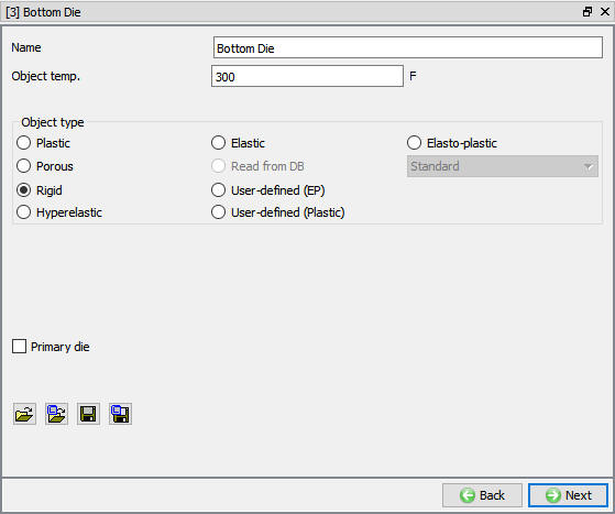
Bottom Die window
Import Geometry
In Geometry page, click on import geometry from library option (![]() ) and import the Spike_BottomDie.STL file from DEFORM installed folder \3d\LABS directory. Use
) and import the Spike_BottomDie.STL file from DEFORM installed folder \3d\LABS directory. Use ![]() button to check the Geometry. Click on
button to check the Geometry. Click on ![]() option, define planar symmetry and click
option, define planar symmetry and click ![]() (see Fig. 3DL3.29.) Click
(see Fig. 3DL3.29.) Click ![]() .
.
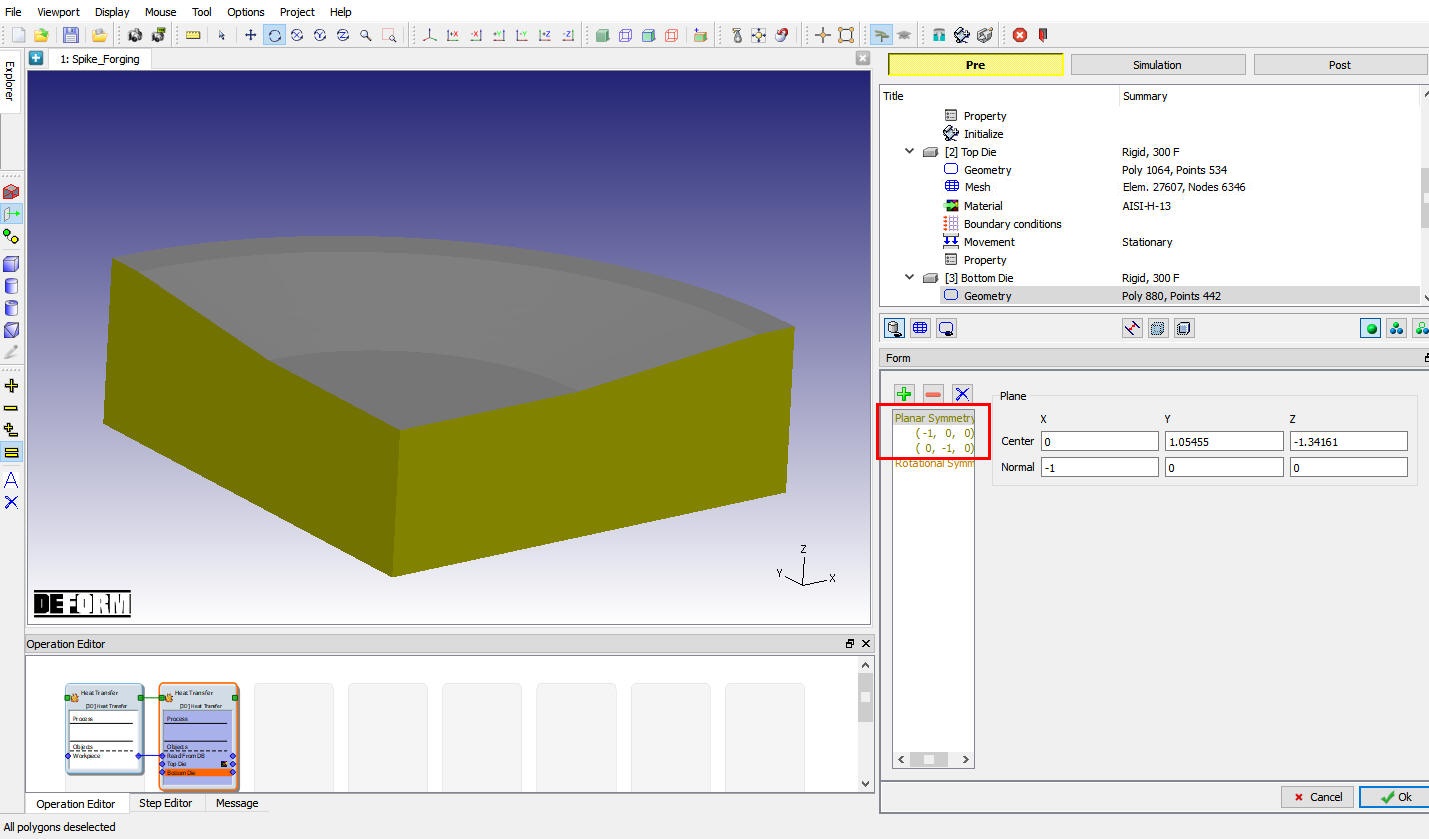
Bottom Die Plane symmetry page
Generate Mesh
Click on ![]() button, select
button, select ![]() in Default Boundary condition popup, a mesh with 30500 elements is generated. Click
in Default Boundary condition popup, a mesh with 30500 elements is generated. Click ![]() .
.
Assigning material Data
Select the AISI-H-13 material from Material list to assign it to Bottom Die as shown in Fig. 3DL3.26. Click ![]() .
.
Assigning BCC
Assigned Default Heat Exchange with Environment Boundary conditions for Bottom die are OK, see Fig. 3DL3.30. Click ![]() until scheduled positioning page.
until scheduled positioning page.
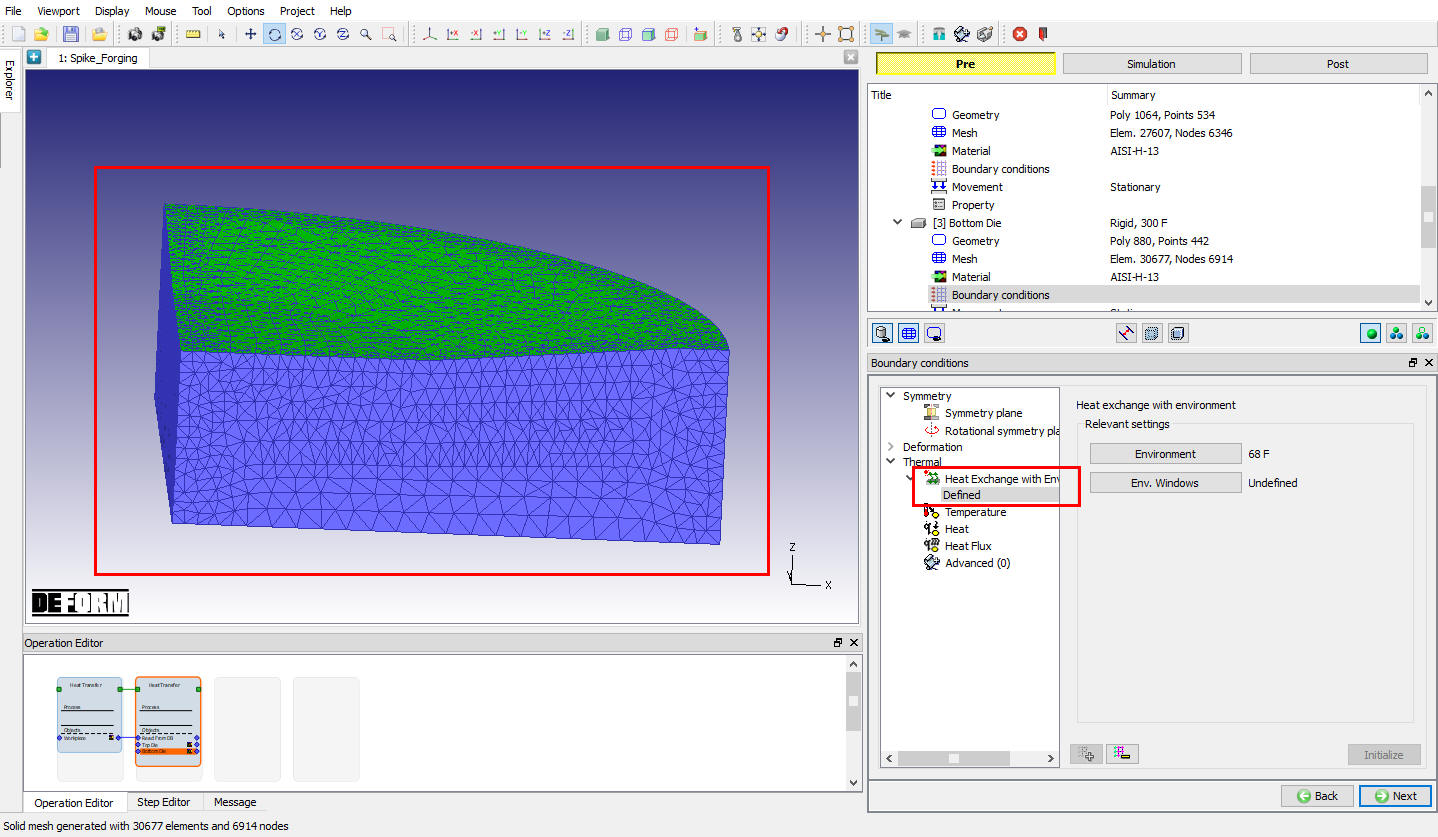
Assigned Heat exchange Boundary conditions for Bottom Die
Scheduled Positioning
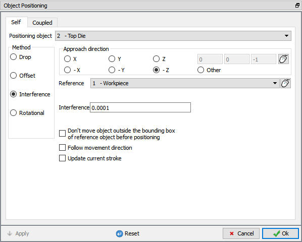
Workpiece needs to be positioned so that it is resting on top of the Bottom Die. Since workpiece is read from DB type, it needs to be positioned by scheduled positioning. To schedule position click on ![]() button and select
button and select ![]() . Change the Positioning Object to the Workpiece and the Reference to the BottomDie. Select the Approach Direction to-Z as shown in Fig. 3DL3.31. and then click
. Change the Positioning Object to the Workpiece and the Reference to the BottomDie. Select the Approach Direction to-Z as shown in Fig. 3DL3.31. and then click ![]() . Defined scheduled positioning will appears as shown in Fig. 3DL3.32. and click on
. Defined scheduled positioning will appears as shown in Fig. 3DL3.32. and click on ![]() .
.
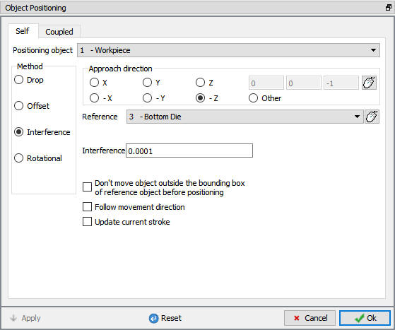
Object positioning Window
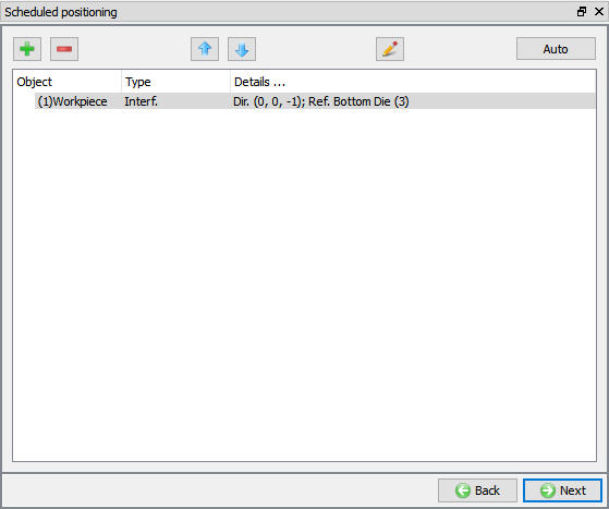
Scheduled Positioning window
Inter-Object relations
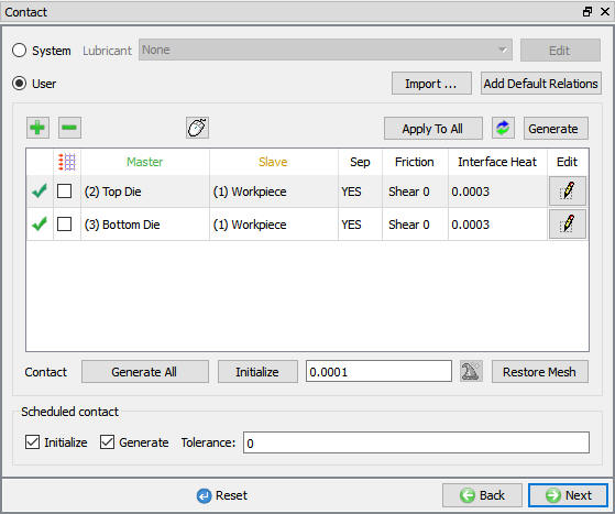
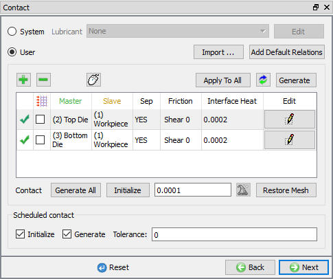
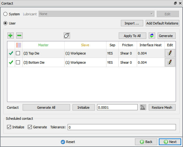
Select user type contact and click on ![]() button. It will add the relationship between the Workpiece, Top Die and Bottom Die as shown in Fig. 3DL3.33.
button. It will add the relationship between the Workpiece, Top Die and Bottom Die as shown in Fig. 3DL3.33.
Inter-object relations window
Highlight the Bottom Die – Workpiece relationship and click the ![]() button to modify the relationship. In the friction section of the screen (see Fig. 3DL3.34.), there is a pull-down menu that allows the user to choose the appropriate friction conditions of Heat transfer processes. Under Thermal tab select Free Resting type Heat transfer coefficient in List. 0.0002 value will be added to Heat transfer coefficient field.
button to modify the relationship. In the friction section of the screen (see Fig. 3DL3.34.), there is a pull-down menu that allows the user to choose the appropriate friction conditions of Heat transfer processes. Under Thermal tab select Free Resting type Heat transfer coefficient in List. 0.0002 value will be added to Heat transfer coefficient field.
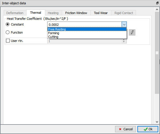
Inter Object Relation Thermal page
Click ![]() to go back to Inter-Object window, since the Problem setup type is Batch mode Contact will generate while generating Database. Click
to go back to Inter-Object window, since the Problem setup type is Batch mode Contact will generate while generating Database. Click ![]() until Step page.
until Step page.
Inter object relation window
Setting Simulation Controls
In Step Definition, Set the Number of steps to 10 , the Step Increment to 5 and Solution step definition Time to0.2 sec (see Fig. 3DL3.36.). Click ![]() .
.
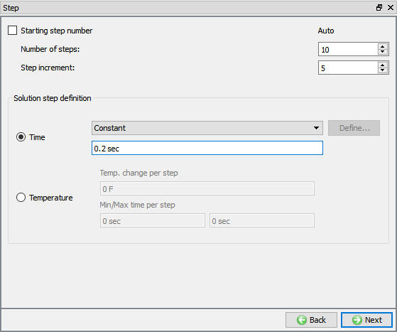
Step controls window
Generate Database
When we visit Generate Database page, objects will be positioned as per defined Scheduled positioning data (see Fig. 3DL3.37.).
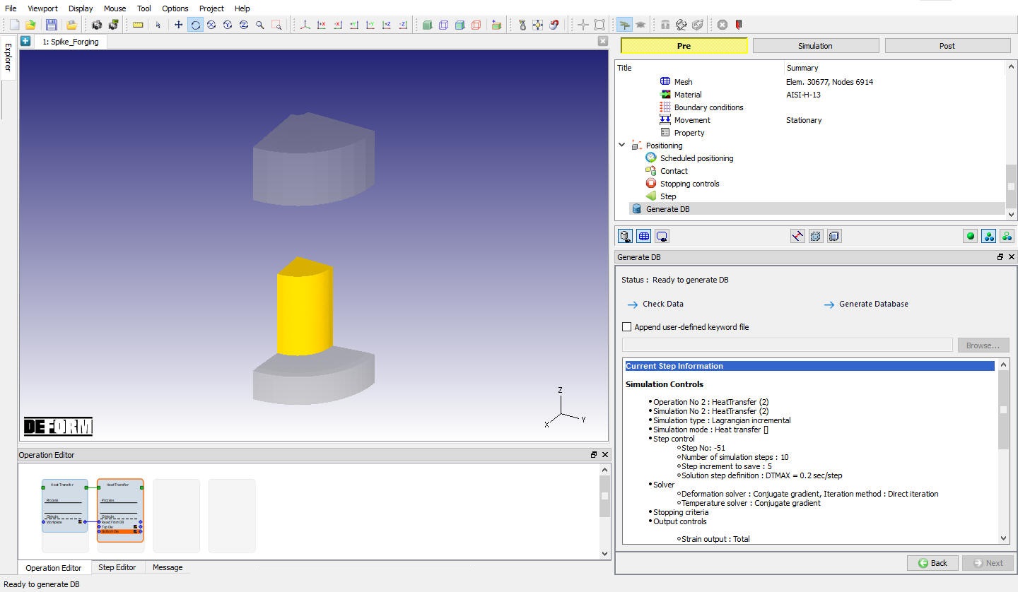
Generate Database
By selecting the File menu ![]() Export** option, Save the Keyword File as “Spike_Dwelling** “.
Export** option, Save the Keyword File as “Spike_Dwelling** “.
Click on ![]() action label to check the problem. Generate database by clicking
action label to check the problem. Generate database by clicking ![]() action label.
action label.
Once the database has been generated, switch to the Simulation mode by selecting the ![]() button above the object tree. Click on the
button above the object tree. Click on the ![]() action label under the simulation tab, Run Options dialog will open as shown in Fig. 3DL3.38.. Use the default Continue Run option to select “Continue from the last step ” option and then select the Simulation mode as Interactive and click on
action label under the simulation tab, Run Options dialog will open as shown in Fig. 3DL3.38.. Use the default Continue Run option to select “Continue from the last step ” option and then select the Simulation mode as Interactive and click on ![]() button to run the simulation.
button to run the simulation.
Run Simulation Popup
Monitor the progress of the simulation by looking at the Simulation Message and Simulation Log tab, making sure that the ![]() option is checked.
option is checked.
Post processing
When the simulation has finished, click on ![]() . In Step Browser click
. In Step Browser click ![]() on button to view all steps.
on button to view all steps.
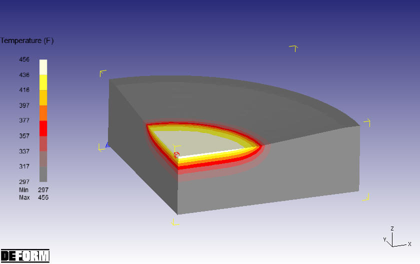
To better view the chilling of the workpiece on the die, select the workpiece in the Object Tree and click the Single object mode ![]() icon. Only the workpiece will be shown in the DISPLAY window. Select Temperature (
icon. Only the workpiece will be shown in the DISPLAY window. Select Temperature (![]() ) state variable and right-click on the Color Bar and select Temperature as the Color Bar Type. (See Fig. 3DL3.39.)
) state variable and right-click on the Color Bar and select Temperature as the Color Bar Type. (See Fig. 3DL3.39.)
Temperature state variable plot for workpiece
Play through the steps of the simulation to look at the workpiece temperature. At Step -51, the position of the workpiece will shift downward where it was rested on the bottom die. Note how the base of the workpiece chills from Step -51 to Step 60 where it is in contact with the die. Turn on the Bottom Die and look at it’s temperature distribution. Observe how the die heats up during the 2 second dwell. (See Fig. 3DL3.40.)
Temperature State variable plot for bottom Die
Now, select last step in Step browser and click on ![]() button to continue the setup.
button to continue the setup.
Spike Forging - Forging Blow1
In the previous operations, the workpiece underwent furnace transfer and dwell on the bottom die. The last step of the Dwell will be loaded into the Pre-processor mode and the first forging blow will be set up.
Add 3D Forming operation from the Explorer Operations list. Add the operation by clicking on 3D Forming ![]() button or can also be added by drag and drop into the Operation editor as shown in Fig. 3DL3.41. Select Forming operation from Operation editor, Setup type popup will appear and click on
button or can also be added by drag and drop into the Operation editor as shown in Fig. 3DL3.41. Select Forming operation from Operation editor, Setup type popup will appear and click on ![]() button in Popup. Click
button in Popup. Click ![]() until objects page.
until objects page.
Adding Forming operation to the Operation Editor
Add objects
By default the three objects from the previous operation will be displayed. If not, by selecting ![]() button, add three objects as shown in Fig. 3DL3.42. Click
button, add three objects as shown in Fig. 3DL3.42. Click ![]() .
.
Adding Objects
Workpiece
In workpiece page, select “Read from DB “ radio button as shown in Fig. 3DL3.43. Since it is a read from DB object, all the data of this object will be carried over to this operation from previous operations. Click ![]() until Top Die page.
until Top Die page.
Selecting Workpiece as read from DB
Top Die
In Top Die page, select “Read from DB “ radio button. Click ![]() until Movement page.
until Movement page.
Assigning Die Movement
**In Movement Page, Set aSpeed** of 2 in/sec in the -Z Direction as shown in Fig. 3DL3.44. Click ![]() until Bottom Die page.
until Bottom Die page.
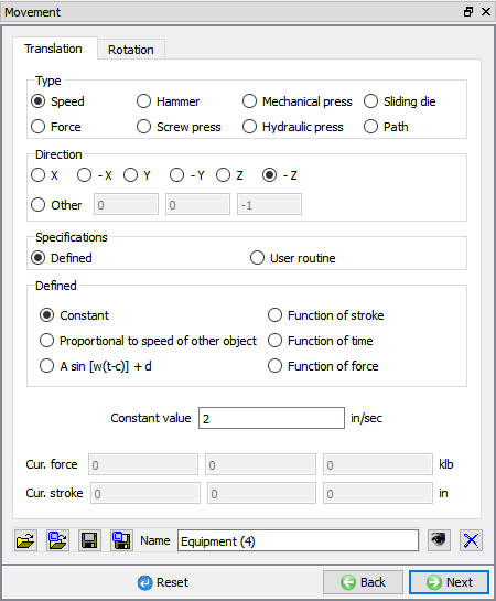
Movement control window
Bottom Die
In Bottom Die page, select “Read from DB “ radio button. Click ![]() until Scheduled positioning page.
until Scheduled positioning page.
Scheduled Positioning the Top Die
In Scheduled positioning page, Click on ![]() button and select
button and select ![]() radio button. Change the Positioning Object to the Top Die and the Reference to the workpiece. Change the Approach Direction to -Z and then click
radio button. Change the Positioning Object to the Top Die and the Reference to the workpiece. Change the Approach Direction to -Z and then click ![]() (see Fig. 3DL3.45.) Click
(see Fig. 3DL3.45.) Click ![]() .
.
Scheduled positioning window
Inter-Object relations
In Inter-Object window, click on ![]() button. Default relations get added as shown in Fig. 3DL3.46.
button. Default relations get added as shown in Fig. 3DL3.46.
Inter-Object window
The Thermal data needs to be modified so that a Forming heat transfer coefficient is used instead of the Free resting coefficient used in the previous operation. The default heat transfer coefficient for hot forming is added automatically which is used in this lab.
Friction needs to be defined between the workpiece and the dies since deformation will now be occurring. Highlight the first relationship in the table and click ![]() . On the Deformationtab , use the friction pull-down menu to select Hot forging (lubricated) from the list as shown in Fig. 3DL3.47., then click on Thermaltab and Select Forming in pull down menu (see Fig. 3DL3.48.), then click
. On the Deformationtab , use the friction pull-down menu to select Hot forging (lubricated) from the list as shown in Fig. 3DL3.47., then click on Thermaltab and Select Forming in pull down menu (see Fig. 3DL3.48.), then click ![]() . Back in the INTER-OBJECT window, click on
. Back in the INTER-OBJECT window, click on ![]() to change the other relationship to these settings.
to change the other relationship to these settings.
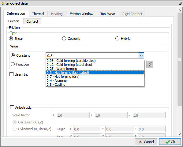
Inter-Object Data Deformation definition Window
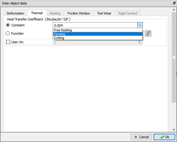
Inter-Object Data Thermal definition Window
Contact will be generated while generating Database, Click ![]() until Step page.
until Step page.
Assigning Step Controls
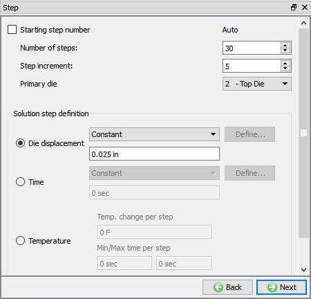
Set the Number of Simulation Steps to 30 and the Step Increment to Save to 5. Change the Primary Die to the TopDie since it is the Top Die that is moving, and under Solution Steps Definition, set With Constant Die Displacement to 0.025 “ as shown in Fig. 3DL3.49. Click ![]() .
.
Simulation Step controls window
Database Generation
By selecting the File menu ![]() Export option, Save a keyword file for the problem as “Spike_Forging_Blow1 “.
Export option, Save a keyword file for the problem as “Spike_Forging_Blow1 “.
Click on ![]() action label to check the problem. Generate a database by clicking
action label to check the problem. Generate a database by clicking ![]() action label.
action label.
Running Simulations
Once the database has been generated, switch to the Simulation mode by selecting the ![]() button above the object tree. Click on the
button above the object tree. Click on the ![]() action label under the simulation tab, Run Options dialog will open as shown in Fig. 3DL3.38.. Use the default Continue Run option to select “Continue from the last step ” option and then select the Simulation mode as Interactive and click on
action label under the simulation tab, Run Options dialog will open as shown in Fig. 3DL3.38.. Use the default Continue Run option to select “Continue from the last step ” option and then select the Simulation mode as Interactive and click on ![]() button to run the simulation.
button to run the simulation.
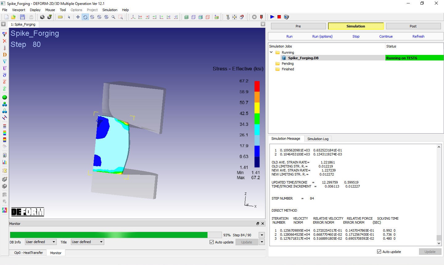
Monitor the progress of the simulation by looking at the Simulation Message and Simulation Log tab, making sure that the ![]() option is checked.
option is checked.
While the simulation is running, the recent saved step can be viewed. Many different variables can be viewed such as plastic strain, plastic strain rate, temperature, etc… from state variables tool bar as shown in Fig. 3DL3.50.
Simulation Graphics window
Post processing
When the simulation has finished, click on ![]() . In Step Browser click on
. In Step Browser click on ![]() button to view all steps.
button to view all steps.
Look at both Temperature and EffectiveStrain as shown in Fig. 3DL3.51. and Fig. 3DL3.52. Depending on the variable being viewed, user may want to toggle between the geometry and the mesh on the dies. When viewing Temperature, the mesh/temperature gradient in the dies can be shown by clicking the Show Mesh ![]() button (and also clicking the Show Geo
button (and also clicking the Show Geo ![]() button to toggle off the geometry). Likewise, when viewing a variable like Effective Strain that only deforming objects would have, the geometries of the dies should probably be viewed instead of the mesh.
button to toggle off the geometry). Likewise, when viewing a variable like Effective Strain that only deforming objects would have, the geometries of the dies should probably be viewed instead of the mesh.
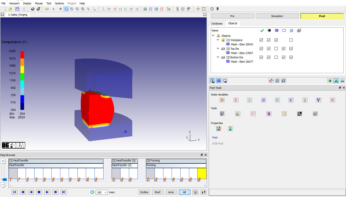
Temperature State variables plot
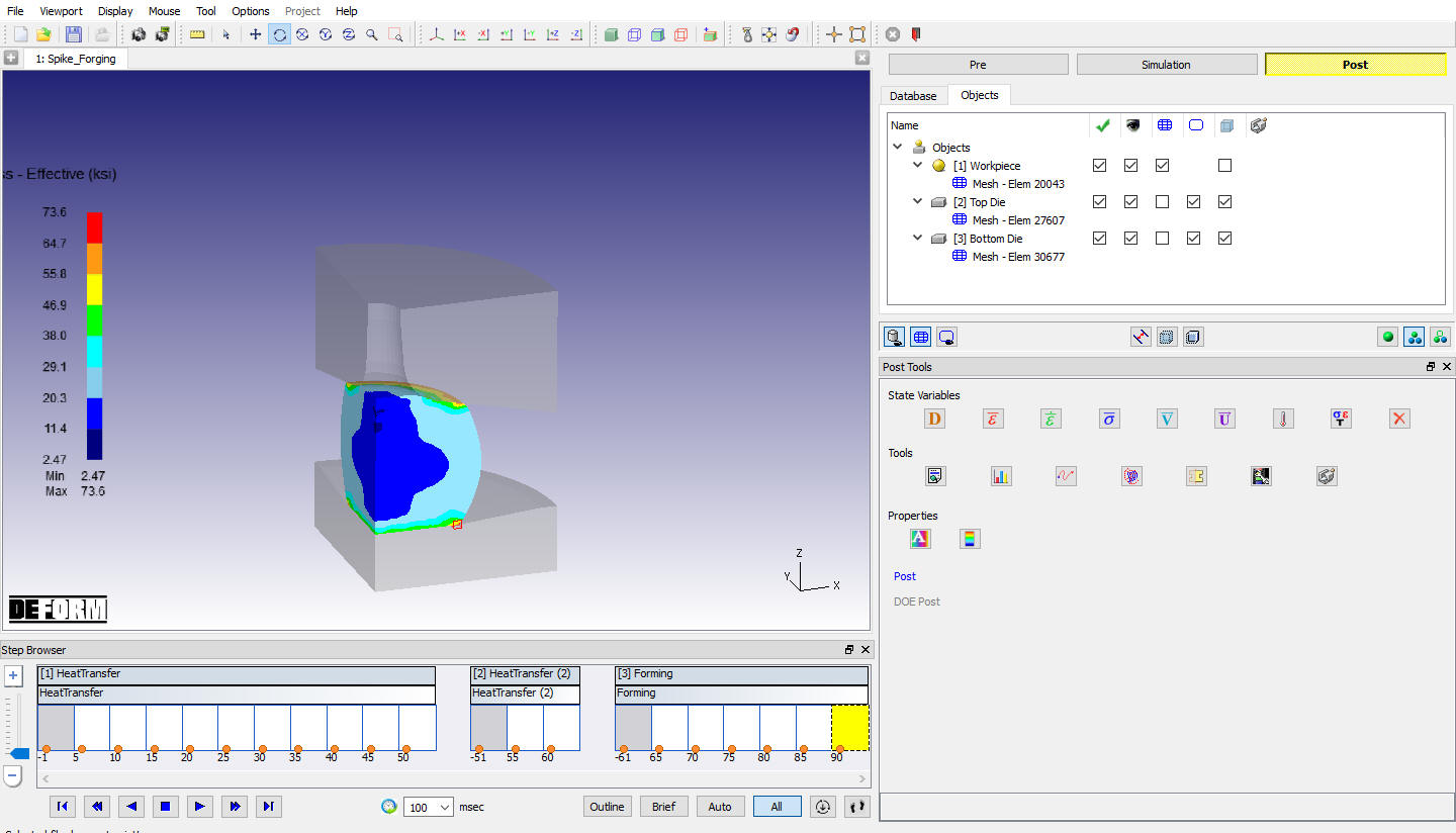
Effective stress State variables plot
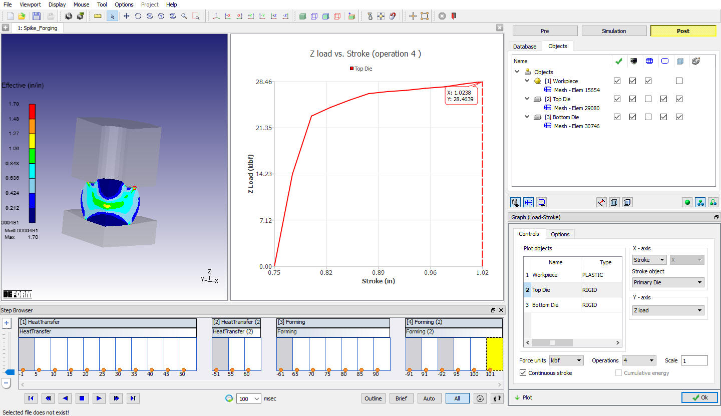
The amount of load required to deform an object is an important result that can be obtained from a simulation. Click on the ![]() icon. When the GRAPH window appears, select only Top Die and the X-Axis is set to Stroke and the Y-Axis is set to Z-Load. Click
icon. When the GRAPH window appears, select only Top Die and the X-Axis is set to Stroke and the Y-Axis is set to Z-Load. Click ![]() and a transparent Load-Stroke curve will display over the objects in the DISPLAY window as shown in Fig. 3DL3.53.
and a transparent Load-Stroke curve will display over the objects in the DISPLAY window as shown in Fig. 3DL3.53.
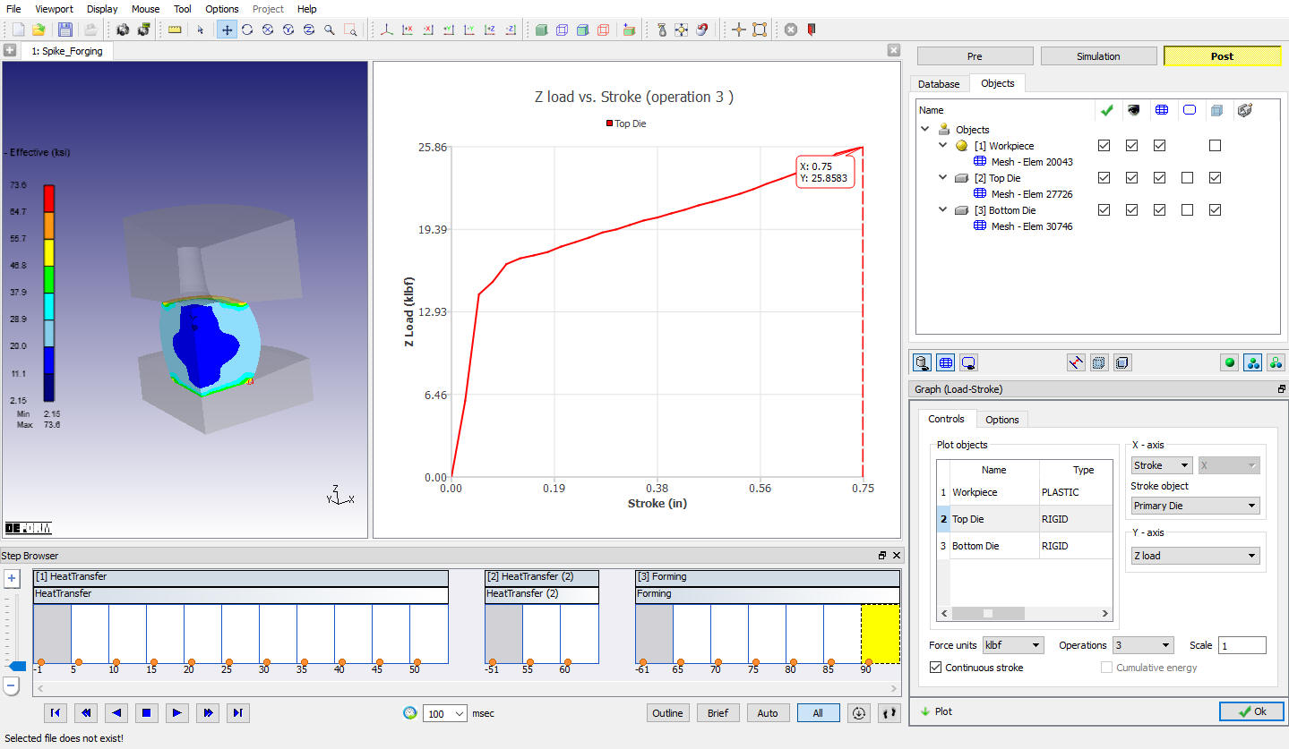
Load Stroke plot
In Load Stroke Graph window, Switch to options tab and check Step tracer check box as shown in Fig. 3DL3.54.
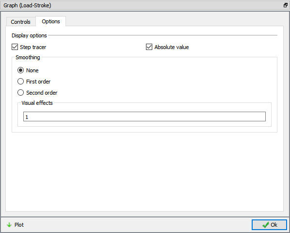
Load Stroke Graph Options window
So that, when a different step is selected, the bar in the Load-Stroke curve will highlight that step and the load for that step will be shown in the graph. Also, a point on the graph can be picked with the mouse and the displayed step will automatically change to the one corresponding to that point on the graph.
Now select last step in Step browser and click on ![]() button to continue the setup.
button to continue the setup.
Spike Forging - Die Change and Blow2
The first forging blow has been simulated and it is now time to model the second blow which uses a different top die. The new top die geometry will be imported and the second forging operation will be set up.
Add 3D Forming operation from the Explorer Operations list. Add the operation by clicking on 3D Forming ![]() button or can also be added by drag and drop into the Operation editor. Select Forming operation from Operation editor, Setup type popup will appear and click on NO- Batch mode button in Popup. Click
button or can also be added by drag and drop into the Operation editor. Select Forming operation from Operation editor, Setup type popup will appear and click on NO- Batch mode button in Popup. Click ![]() until objects page.
until objects page.
Add objects
Click ![]() until Objects page. By default the three objects from the previous operation will be displayed. If not, by selecting
until Objects page. By default the three objects from the previous operation will be displayed. If not, by selecting ![]() button, add three objects as shown in Fig. 3DL3.42. Click
button, add three objects as shown in Fig. 3DL3.42. Click ![]() .
.
Workpiece
In workpiece page, select “Read from DB “ radio button. Click ![]() until Top Die page.
until Top Die page.
Changing Top die for Blow2
Both the geometry and mesh of the top die have to be changed. In Top Die page, change Object type to rigid and assign temperature as 300 °F then Click ![]() .
.
Import Geometry
In Geometry page, click on import geometry from library option (![]() ) and import the Spike_Topdie2.STL file file from DEFORM installed folder \3d\LABS directory. Use
) and import the Spike_Topdie2.STL file file from DEFORM installed folder \3d\LABS directory. Use ![]() button to check the Geometry. Click on
button to check the Geometry. Click on ![]() option, define planar symmetry and Click
option, define planar symmetry and Click ![]() (see Fig. 3DL3.55.) Click
(see Fig. 3DL3.55.) Click ![]() .
.
Assigned Plane Symmetry for Top Die
Generate Mesh
Click on ![]() button, select
button, select ![]() in Default Boundary condition popup. A mesh with default number of elements will be generated.
in Default Boundary condition popup. A mesh with default number of elements will be generated.
Assign Material
Select the material ‘AISI-H-13 ‘ material from material window and assign it to the Top Die. Click on ![]() .
.
Assigning BCC
In BCC page, Check the default assigned Heat exchange with Environment BCC for Top Die and make sure that default assigned Heat Exchange with Environment BCC is assigned to the entire outer surface of the top die except the symmetry planes (see Fig. 3DL3.56.).
Assigning Heat Exchange with Environment BCC for Top Die
Assigning Die Movement
In Movement Page, Set a Speed of 2 in/sec in the -Z Direction. Click ![]() .
.
Bottom Die
In Bottom Die page select “Read from DB “ radio button. Click ![]() .
.
Scheduled Positioning the Top Die
In Scheduled positioning page, Click on ![]() button and select
button and select ![]() radio button. Change the Positioning Object to the TopDie and the Reference to the workpiece. Change the Approach Direction to-Z and then click
radio button. Change the Positioning Object to the TopDie and the Reference to the workpiece. Change the Approach Direction to-Z and then click ![]() . Click
. Click ![]() .
.
Inter-Object relations
In Inter-Object window, click on ![]() button. Default relations get added as shown in Fig. 3DL3.47.
button. Default relations get added as shown in Fig. 3DL3.47.
Friction needs to be defined between the workpiece and the dies since deformation will now be occurring. Also, the Thermal data needs to be modified so that a Forming heat transfer coefficient is used instead of the Free resting coefficient used in the previous operation.
Highlight the first relationship in the table and click ![]() . On the Deformation tab, use the friction pull-down menu to select Hot forging (lubricated) from the list as shown in Fig. 3DL3.48. then click
. On the Deformation tab, use the friction pull-down menu to select Hot forging (lubricated) from the list as shown in Fig. 3DL3.48. then click ![]() . Back in the INTER-OBJECT window, click on
. Back in the INTER-OBJECT window, click on ![]() to change the other relationship to these settings.
to change the other relationship to these settings.
Contact will be generated between the Billet and both the Top and Bottom Dies while generating Database.
Click ![]() up to Step controls page.
up to Step controls page.
Assigning Step Controls
Set theNumber of Simulation Steps to 10 and the Step Increment to Save to 5. Change the Primary Die to the Top Die since it is the Top Die that is moving, and under Solution Steps Definition, set With Constant Die Displacement to 0.025 “. Click![]() .
.
Database Generation
By selecting the Filemenu ![]() Export** option, Save a keyword file for the problem as “Spike_Forging_Blow2** “.
Export** option, Save a keyword file for the problem as “Spike_Forging_Blow2** “.
Click on ![]() action label to check the problem. Generate a database by clicking
action label to check the problem. Generate a database by clicking ![]() action label.
action label.
Once the database has been generated, switch to the Simulation mode by selecting the ![]() button above the object tree. Click on the
button above the object tree. Click on the ![]() action label under the simulation tab, Run Options dialog will open. Use the default Continue Run option to select “Continue from the last step ” option and then select the Simulation mode as Interactive and click on
action label under the simulation tab, Run Options dialog will open. Use the default Continue Run option to select “Continue from the last step ” option and then select the Simulation mode as Interactive and click on ![]() button to run the simulation.
button to run the simulation.
Monitor the progress of the simulation by looking at the Simulation Message and Simulation Log tab, making sure that the ![]() option is checked.
option is checked.
Post processing
When the simulation has finished, click on ![]() . In Step Browser click on
. In Step Browser click on ![]() button to view all steps.
button to view all steps.
Play through the steps, focusing especially on the steps for the second forging blow, Steps-90 to 101. Use the ![]() button to view how the contact evolves through the simulation. Also, investigate temperature, effective strain and load vs. stroke behavior.
button to view how the contact evolves through the simulation. Also, investigate temperature, effective strain and load vs. stroke behavior.
Load-stroke Window with effective strain state variable plot