Lab 2: 2D Heat Treatment Wizard
2.1. Introduction
2.2. Starting a New problem
2.3. Defining Process Settings
2.4. Loading Material definition
2.5. Defining Workpiece
2.5.1. Workpiece General Object
2.5.2. Import Geometry for workpiece
2.5.3. Assigning Material
2.5.4. Generate Mesh
2.5.5. Assigning Boundary conditions
2.5.6. Workpiece initialization
2.6. Medium Definition
2.7. Scheduled Definition
2.8. Simulation controls
2.9. Generate Database
2.10. Starting the Simulation
2.11. Post processing
Introduction
The Heat Treatment Wizard is a convenient tool to set up complex multiple-operation heat treatment problem. This lab will demonstrate how to use this wizard to prepare a carburization-quench-tempering simulation of a steel part. This lab can also help users understand the capabilities of DEFORM-HT’s phase transformation calculation scheme.
Starting a New problem
On a Windows machine , go to the ![]() button select DEFORM-v1x.xxx (.xxx indicates version number E.g. v14.0.2) and select DEFORM GUI Main vxx.xx from the menu. The DEFORM GUI Main window will appear.
button select DEFORM-v1x.xxx (.xxx indicates version number E.g. v14.0.2) and select DEFORM GUI Main vxx.xx from the menu. The DEFORM GUI Main window will appear.
Create a new problem either by selecting File![]() **New Problem** or by clicking the New Problem
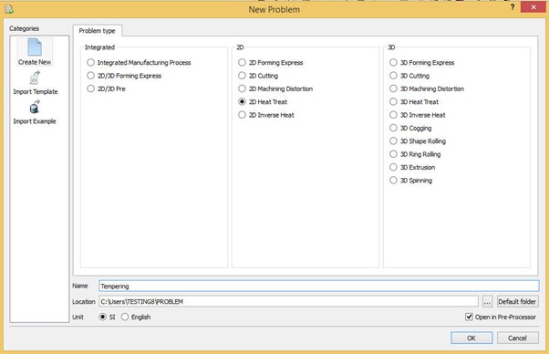
**New Problem** or by clicking the New Problem ![]() icon. The Problem Setup window will appear as shown in Fig. 2DHTWL2.1. Select “ 2D Heat Treat “ radio button and unit system as “SI “ radio button in Units field. Define problem Name as ‘Tempering ’ and make sure the “Show option dialog” check box is turned on (if we do not turn on the “Show option dialog ” check box, then we will not get the New Project dialog in MO UI). Then click on
icon. The Problem Setup window will appear as shown in Fig. 2DHTWL2.1. Select “ 2D Heat Treat “ radio button and unit system as “SI “ radio button in Units field. Define problem Name as ‘Tempering ’ and make sure the “Show option dialog” check box is turned on (if we do not turn on the “Show option dialog ” check box, then we will not get the New Project dialog in MO UI). Then click on ![]() button to open a new Problem using the Deform Integrated Manufacturing Process.
button to open a new Problem using the Deform Integrated Manufacturing Process.
Defining New Problem.
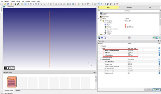
Multiple operation wizard will open with 2D HT operation as first operation as shown in Fig. 2DHTWL2.2.
New project with 2D HT Operation.
Defining Process Settings
As the multiple operation wizard opens, Process settings page will be displayed in property editor region as shown in Fig. 2DHTWL2.2. User can set the simulation mode based on the simulation requirement along with step definition controls. For this lab, we will turn on “Deformation “, “Diffusion “ and “PhaseTransformation “. Step definition will be defined in Simulation controls page. Click ![]() until Material list page, as we do not need to make any changes in Initialization page.
until Material list page, as we do not need to make any changes in Initialization page.
Loading material to Material list
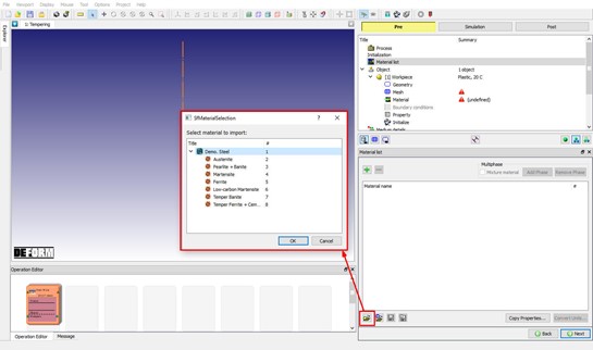
In Material list page, click on ![]() (Import material from file) and import material “Demo_Temper_Steel.KEY “ from installation path \SFTC\DEFORM\v_\2d\LABS\HeatTreat directory (See Fig. 2DHTWL2.3.). Click
(Import material from file) and import material “Demo_Temper_Steel.KEY “ from installation path \SFTC\DEFORM\v_\2d\LABS\HeatTreat directory (See Fig. 2DHTWL2.3.). Click ![]() to material Selection popup dialog, we can observe that material has multiple phases defined and we can observe each phase material properties using
to material Selection popup dialog, we can observe that material has multiple phases defined and we can observe each phase material properties using ![]() button to navigate to respective phase. Click
button to navigate to respective phase. Click ![]() until Workpiece object page.
until Workpiece object page.
Importing Material into Material list page.
Defining Workpiece
Workpiece general object definition
In Workpiece page, change the object type to Elasto-plastic type and click ![]() (See Fig. 2DHTWL2.4.)
(See Fig. 2DHTWL2.4.)
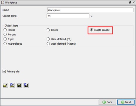
Workpiece general object definition.
Importing Geometry for Workpiece
In Geometry page, click on ![]() (import geometry from library) option and import the “TemperingPart.GEO ” file from installation path \SFTC\DEFORM\v_\2d\LABS\HeatTreat as shown in Fig. 2DHTWL2.5. Use
(import geometry from library) option and import the “TemperingPart.GEO ” file from installation path \SFTC\DEFORM\v_\2d\LABS\HeatTreat as shown in Fig. 2DHTWL2.5. Use ![]() action label to check the imported geometry. If they are any issues with the geometry then geometry will be corrected and message will be displayed as shown in Fig. 2DHTWL2.6. Click
action label to check the imported geometry. If they are any issues with the geometry then geometry will be corrected and message will be displayed as shown in Fig. 2DHTWL2.6. Click ![]() until Material page.
until Material page.
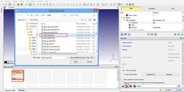
Importing Geometry for Workpiece.
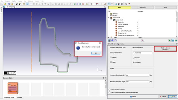
Fixing geometry errors in imported geometry.
Assigning Material to Workpiece
In Material page, select Demo.Steel from material list to assign the material to workpiece as shown in Fig. 2DHTWL2.7. Click ![]() to Mesh page.
to Mesh page.
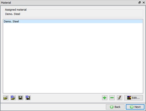
Assigning Material to workpiece.
Generating Mesh for Workpiece
In Mesh page, define Target number of mesh elements as 300. We need to define structured mesh for better prediction of phase distribution and atom content on surface, hence click on ![]() to toggle mesh settings into expert mode, select Coating mesh and add 2 layers of coating as shown in Fig. 2DHTWL2.9. Set “Thickness mode “ to be “ratio to object overall dimension “ and define 500 microns and 1000microns as thickness for layer 1 and 2 respectively as shown in See Fig. 2DHTWL2.9. , we will keep default selection of “Demo.Steel ” as material for coating. Click on
to toggle mesh settings into expert mode, select Coating mesh and add 2 layers of coating as shown in Fig. 2DHTWL2.9. Set “Thickness mode “ to be “ratio to object overall dimension “ and define 500 microns and 1000microns as thickness for layer 1 and 2 respectively as shown in See Fig. 2DHTWL2.9. , we will keep default selection of “Demo.Steel ” as material for coating. Click on ![]() . Mesh generated for Workpiece along with structured mesh looks like as shown in Fig. 2DHTWL2.9. Click on
. Mesh generated for Workpiece along with structured mesh looks like as shown in Fig. 2DHTWL2.9. Click on ![]() to toggle to guided mode. Click
to toggle to guided mode. Click ![]() until Boundary condition page.
until Boundary condition page.
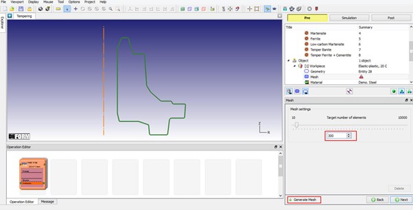
Defining number of elements for Workpiece mesh.
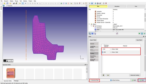
Coating mesh settings for Workpiece.
Assigning Boundary conditions to Workpiece
In Boundary conditions page, we will fix nodes in Y direction on bottom edge of the Workpiece as shown in Fig. 2DHTWL2.10.. Click ![]() to Initialization page.
to Initialization page.
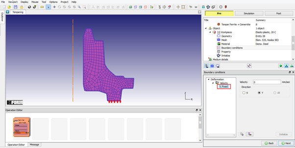
Assigning Velocity BCC to Workpiece.
Initializing Phase distribution and Atom percentage in Workpiece
In Initialization page, click on “Microstructure ” tab and define initial value of “Pearlite+Bainite ” as “1” in 3rd column as shown in Fig. 2DHTWL2.11. and then click on ![]() button to initialize the value for entire Workpiece.
button to initialize the value for entire Workpiece.
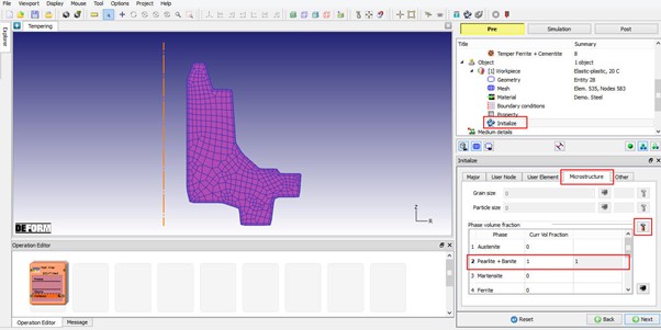
Initializing Phase volume fractions of Workpiece.
To initialize atom content, click on NodeData![]() **and select “Diffusion** ” tab to initialize atom content value as shown in Fig. 2DHTWL2.12. Click on
**and select “Diffusion** ” tab to initialize atom content value as shown in Fig. 2DHTWL2.12. Click on ![]() , “Initialize Nodal data” pop-up will open, select “Range” and let range of nodes be default selection of all nodes at Start Node and End Node. Define “Value” as 0.2 and click on
, “Initialize Nodal data” pop-up will open, select “Range” and let range of nodes be default selection of all nodes at Start Node and End Node. Define “Value” as 0.2 and click on ![]() button to initialize value, see Fig. 2DHTWL2.12. Click on
button to initialize value, see Fig. 2DHTWL2.12. Click on ![]() to close the “Initialize Nodal data” and click on
to close the “Initialize Nodal data” and click on ![]() to close Nodal data dialog. Click
to close Nodal data dialog. Click ![]() to define Medium details.
to define Medium details.
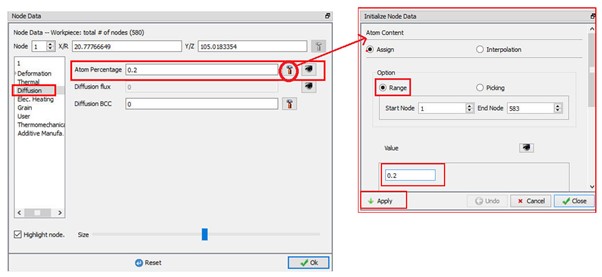
Initializing Atom content for Workpiece.
Medium Definition for heat treatment
In page “Mediumdetails ”, we will define various media and heat transfer zones associated with them,
1. Rename the first medium to “Furnace ” and set the “Default ” heat transfer coefficient (HTC) to constant 0.1. Turn on Radiation checkbox as shown in Fig. 2DHTWL2.13.
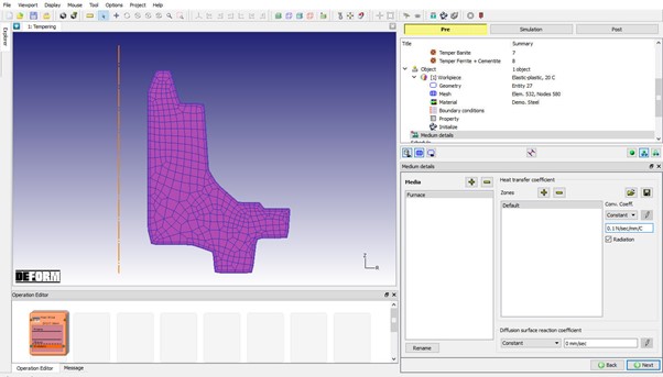
Defining Furnace Medium.
2. Add a medium “Polymer**Solution** ”, turn off Radiation check box and set its “Default “ zone HTC as a function of temperature. Define the function using ![]() button as shown in Table.1. and Fig. 2DHTWL2.14.
button as shown in Table.1. and Fig. 2DHTWL2.14.
| Temperature | HTC |
|---|---|
| 20 | 3.5 |
| 400 | 8.5 |
| 700 | 15 |
| 900 | 5.2 |
Polymer solution HTC function.
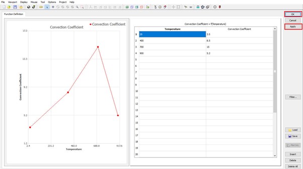
Defining Polymer solution HTC function.
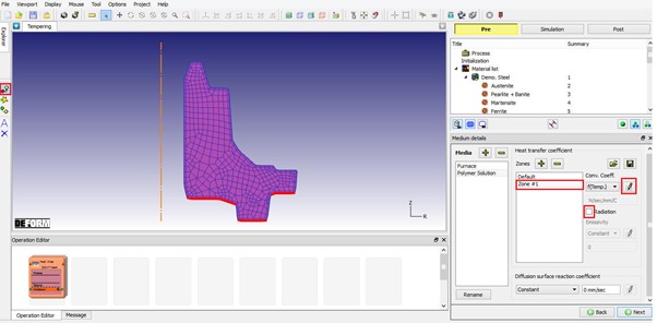
3. Add a heat transfer zone to the “Polymer**Solution** ” medium. Click on the workpiece boundary to specify this zone using the ![]() selection mode as shown in Fig. 2DHTWL2.15. Select HTC as a function of temperature and define the values of function using
selection mode as shown in Fig. 2DHTWL2.15. Select HTC as a function of temperature and define the values of function using ![]() button as shown in Table. 2. and Fig. 2DHTWL2.16.
button as shown in Table. 2. and Fig. 2DHTWL2.16.
Defining Zone 1 of Polymer medium.
| Temperature | HTC |
|---|---|
| 20 | 3.5 |
| 200 | 4.5 |
| 400 | 8.8 |
| 700 | 3.5 |
| 900 | 2.8 |
HTC function of Polymer solution medium Zone 1.
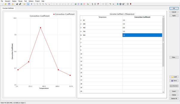
Defining HTC function of Polymer solution medium Zone 1.
4. For Zone1 of “Polymer Solution” medium, select the “Diffusion Surface Reaction Rate” as a function of temperature as shown in Table.3. Define the function as shown in Fig. 2DHTWL2.17. and Fig. 2DHTWL2.18.
| Temperature | RRC |
|---|---|
| 20 | 0.1 |
| 500 | 0.2 |
| 1000 | 0.6 |
Diffusion Surface Reaction Rate function of Polymer solution medium Zone 1
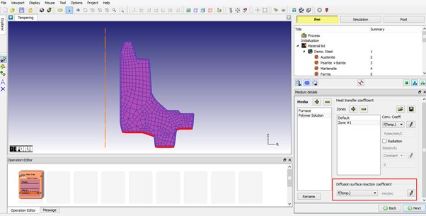
Setting Zone1 Radiation and Diffusion properties.
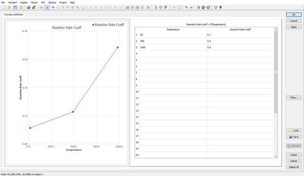
Defining Surface Reaction Rate function of Polymer solution medium Zone 1
5. Add one more media, rename it to “Air”. Define “Default” HTC as 0.02 and turn on Radiation checkbox as shown in Fig. 2DHTWL2.19. Click ![]() to schedule Heat Treatment operations.
to schedule Heat Treatment operations.
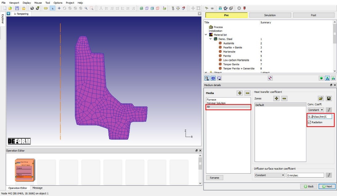
Defining Air medium.
Scheduling heat treatment operations
In this lab we are going to carry out a five stage Heat Treatment process. To do so, in “Schedule ” page, input a five-stage schedule as explained below.
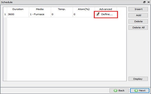
1. One hour (3600 s) of furnace heating. The temperature of the furnace is specified as a function of time. This function can be input by clicking the corresponding “Define” cell in the “Advance” column (See Table.4., Fig. 2DHTWL2.20, Fig. 2DHTWL2.21. and Fig. 2DHTWL2.22.).
| Time(s) | Temperature |
|---|---|
| 0 | 20 |
| 600 | 660 |
| 1200 | 880 |
| 3600 | 880 |
Defining Furnace environment temperature function during Furnace heating operation.
Heat Treatment Process scheduling.
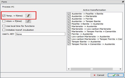
Defining Furnace heating window in Advance
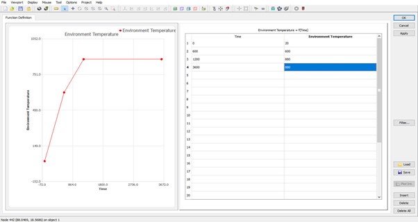
Function definition detail window
2) Schedule second HT operation for10 minutes (600 s) of quenching in the polymer solution. Specify the “Atom” content to be 0.8 at 30C as shown in Fig. 2DHTWL2.23.
3) Schedule third HT operation of tempering as Furnace heating for 30 minutes (1800 s) at temperature 250C as shown in Fig. 2DHTWL2.23.
4) Schedule fourth HT operation of tempering as Furnace heating for 30 minutes (1800 s) at temperature 350C as shown in Fig. 2DHTWL2.23.
5) Schedule fourth HT operation of tempering as cooling in Air for One hour (3600 s) at 20C environment temperature as shown in Fig. 2DHTWL2.23. and click ![]() to Step page.
to Step page.
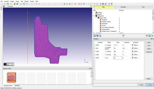
Heat Treatment operations schedule.
Defining Simulation controls
In “Step “ page, select Auto radio button and set “Temp. Change per step “ to 5° C, keep Minimum time per step as 0.001 sec and. Maximum time per step as 10 sec. Define Step increment to save as 10. (See Fig. 2DHTWL2.24.)
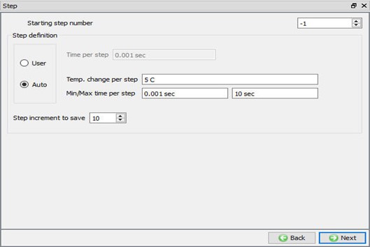
Defining step controls for Heat Treatment simulation.
Generate Database
Click on ![]() action label to check for errors and warnings that need to be addressed before generating database. If there are no errors or warnings that would affect the simulation output, generate a database by clicking
action label to check for errors and warnings that need to be addressed before generating database. If there are no errors or warnings that would affect the simulation output, generate a database by clicking ![]() action label, see Fig. 2DHTWL2.25. When the program is done writing the database, switch to
action label, see Fig. 2DHTWL2.25. When the program is done writing the database, switch to ![]() tab to run simulation.
tab to run simulation.
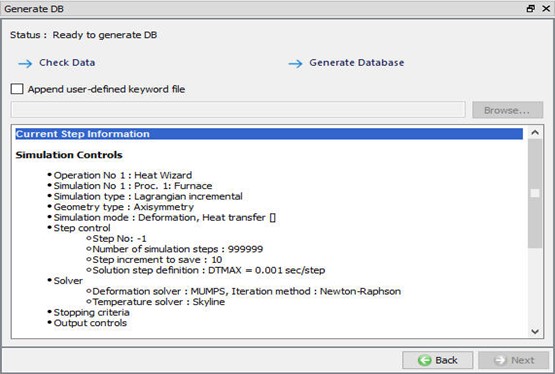
Generating Database
Starting the Simulation
Click on the ![]() action label to open the Run Options dialog as shown in Fig. 2DHTWL2.26. Use the default Continue Run option to select “Continue from the last step ” (from step -1) option and then select the Simulation mode as Interactive and click on
action label to open the Run Options dialog as shown in Fig. 2DHTWL2.26. Use the default Continue Run option to select “Continue from the last step ” (from step -1) option and then select the Simulation mode as Interactive and click on ![]() button to run the simulation.
button to run the simulation.
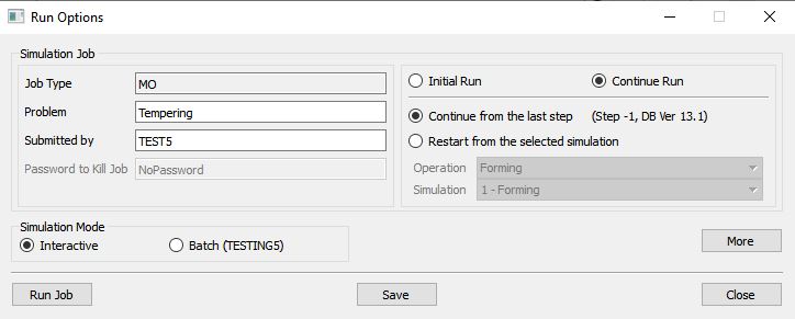
Run simulation window
The progress of the simulation can be monitored as it is running by looking at the Simulation Message and process monitor in Simulation mode. Click the Simulation Message tab to view the Message file. As long as the ![]() option is checked, which is the default setting, the Message file will refresh every couple of seconds.
option is checked, which is the default setting, the Message file will refresh every couple of seconds.
The Message file provides information about which simulation step the simulation is currently on and gives information dealing with how well the simulation is running.
When the simulation of all Heat Treatment operations is finished, the message will be added as shown in Fig. 2DHTWL2.27. to the end of the Message file.
Each stage defined will be executed as individual operation and user need to wait until all the stages simulation is completed.
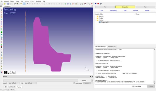
Monitoring Heat Treatment Simulation progress.
Post-Processing
When the simulation has finished, click on ![]() . In Step Browser click on
. In Step Browser click on ![]() button to view all steps. The temperature min-max history should look like the graph below (See Fig. 2DHTWL2.28.).
button to view all steps. The temperature min-max history should look like the graph below (See Fig. 2DHTWL2.28.).
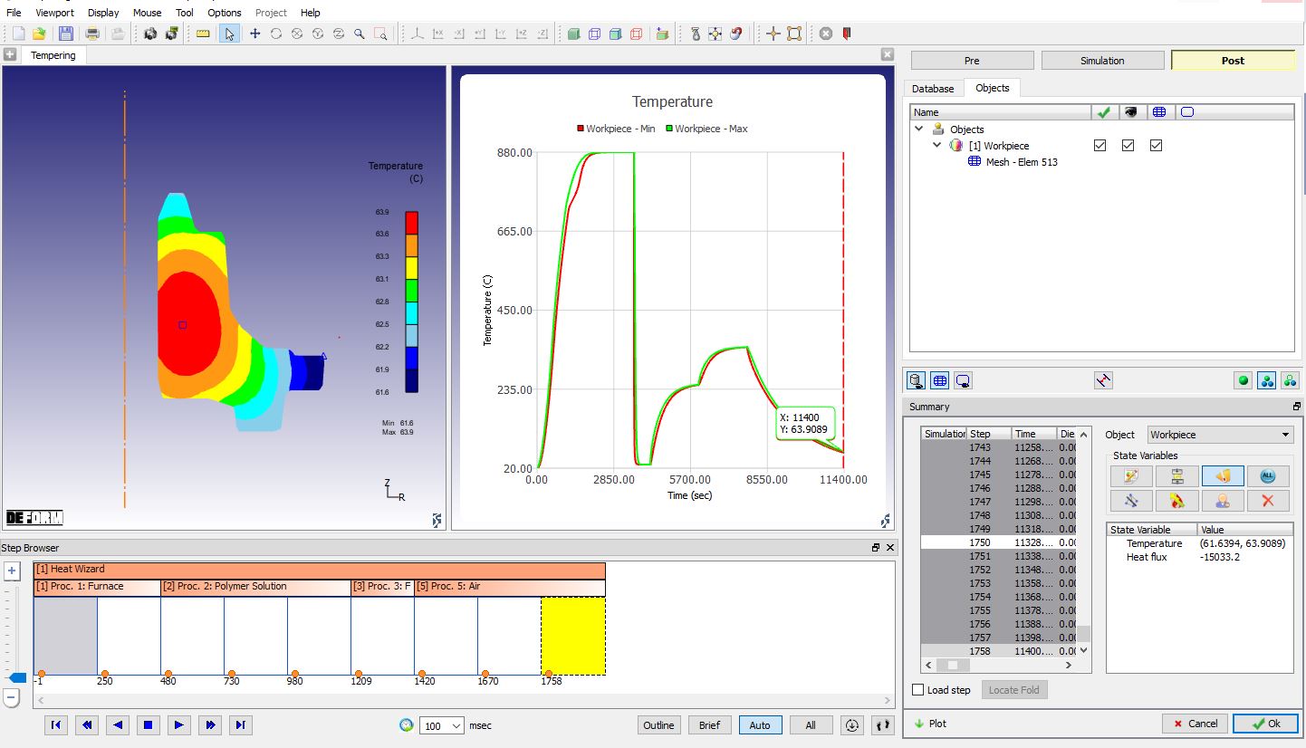
Temperature Min-Max history throughout Heat Treatment simulation.
Plot the Volume fraction of each phases at the end of all operations (See Fig. 2DHTWL2.29.).
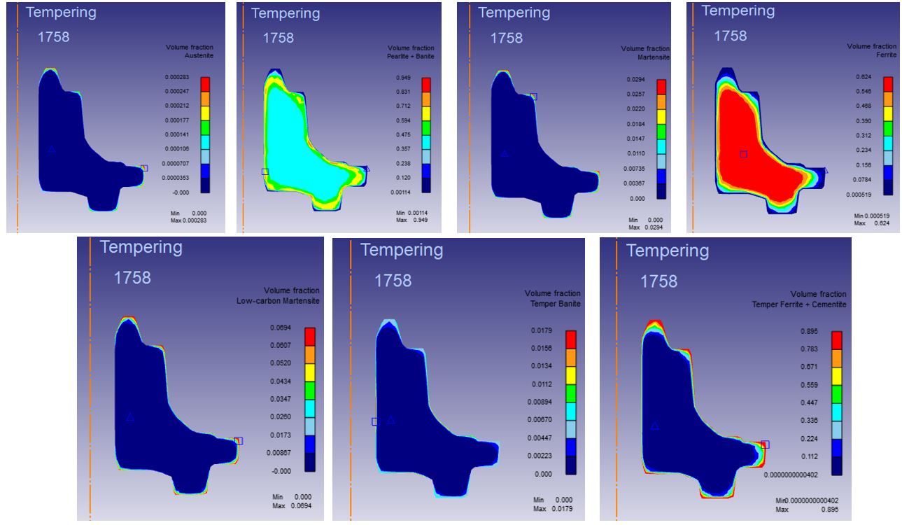
Volume Fraction distribution at the end of all operations.
Plot Dominant atom from Diffusion and observe the Dominant Atom distribution at different stage of Tempering operation (See Fig. 2DHTWL2.30.).
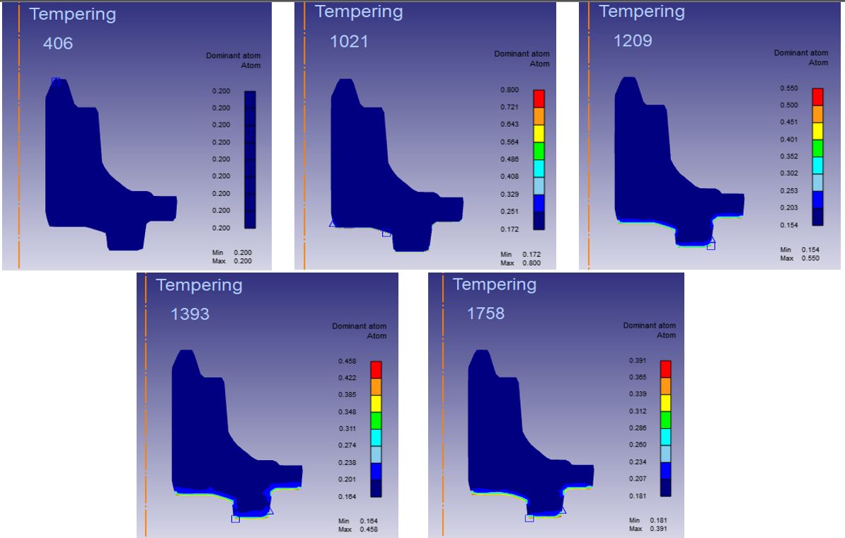
Dominant atom distribution at the end of each operation.