3D Heat Treatment Wizard Lab

1.1. Introduction

1.2. Starting a New problem

1.3. Process Settings

1.4. Material definition

1.5. Workpiece Object Type

1.6. Workpiece initialization

1.7. Medium Definition

1.8. Scheduled Definition

1.9. Simulation controls

1.10. Generate Database

1.11. Starting the Simulation

1.12. Post processing

Introduction

The Heat Treatment Wizard is a convenient tool to set up complex multiple-operation heat treatment problem. This lab will demonstrate how to use this wizard to prepare a carburization-quench-tempering simulation of a steel part. This lab can also help users understand the capabilities of DEFORM-HT’s phase transformation calculation scheme.

Starting a New problem

On a Windows machine , go to the button select DEFORM-v1x.xxx (.xxx indicates version number E.g. v14.0.2) and select DEFORM GUI Main vxx.xx from the menu. The DEFORM GUI Main window will appear as shown in below (see Fig. 3DHTWL1.1.)

DEFORM GUI main window

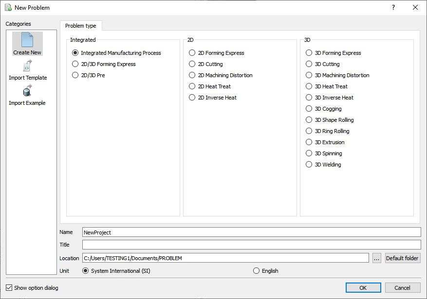
Create a new problem either by selecting File **New Problem** or by clicking the New Problem icon. The Problem Setup window will appear as shown in Fig. 3DHTWL1.2. Select “ Integrated Manufacturing Process “ radio button and units system as “SI “ using radio button. Define Problem Name as “GearHT “ and make sure the “Show option dialog” check box is turned on (if we do not turn on the “Show option dialog ” check box, then we will not get the New Project dialog in MO UI). Then click on button to open a new Problem using the Deform Integrated Manufacturing Process.

Problem type selection window

Integrated Manufacturing Process wizard will open (see Fig. 3DHTWL1.3.), at this point user will be prompted to specify a project name (system will create a separate folder with this project name) and title. In this lab we will use ‘GearHT ’ as the project name.

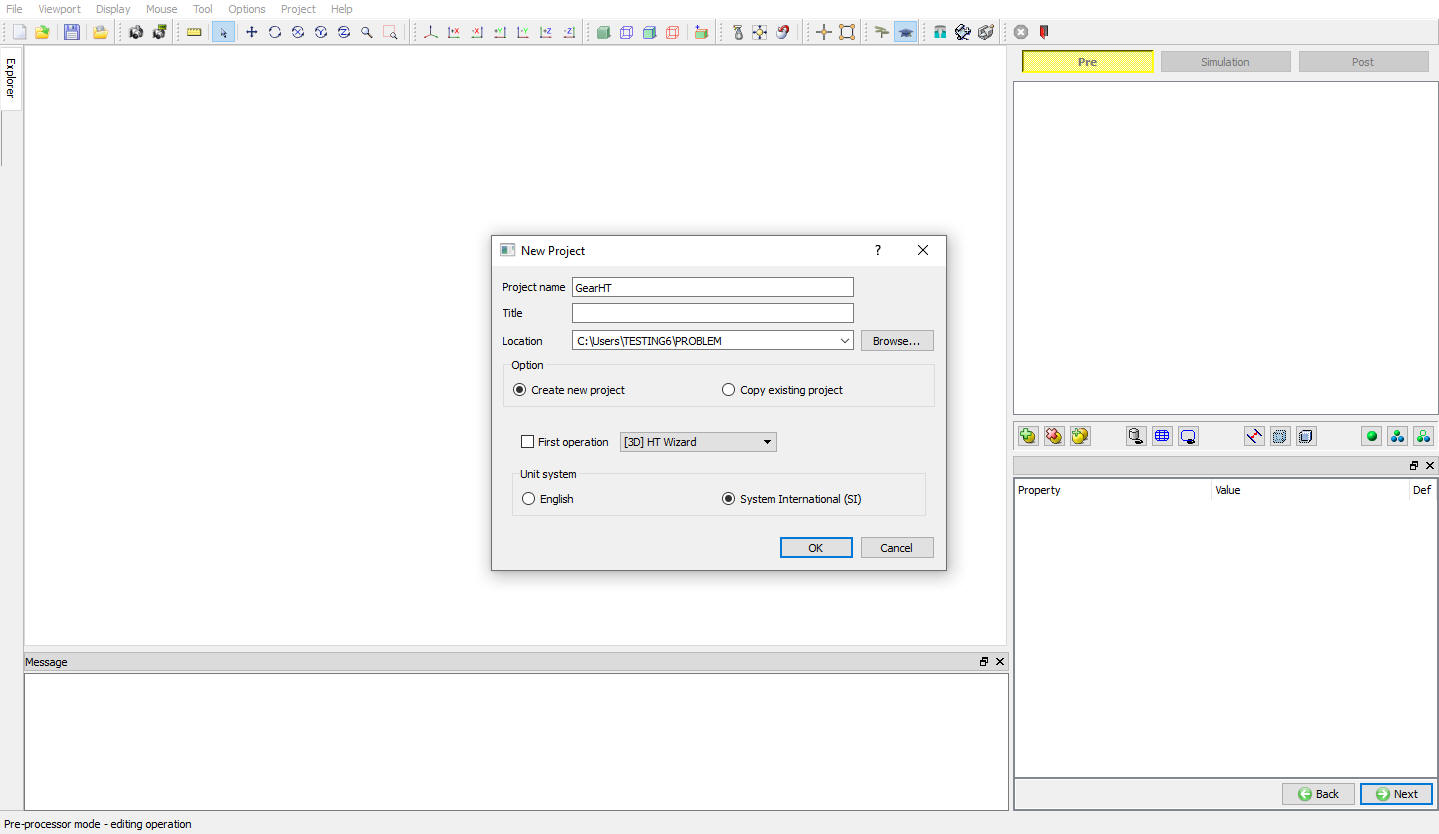
MO wizard New project

User can also change the Unit system (File menu selected unit system will be selected by default) and add HT operation by selecting it from First operation pull down list and checkbox (see Fig. 3DHTWL1.3.). Using copy Existing project option we can import previous saved projects as new project. Click on to continue to open the operation.

Multiple Operation wizard will open. Add 3D HT Wizard operation from the Explorer Operations list. Add the operation by clicking on button next to 3D HT Wizard or user can also add by drag and drop into the Operation Editor (see Fig. 3DHTWL1.4.).

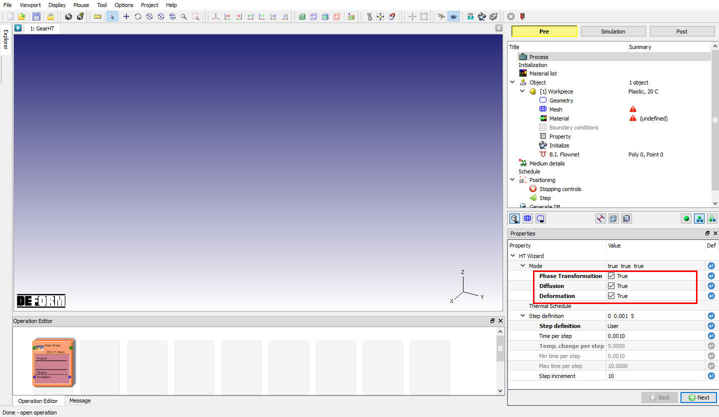
Added 3D HT Wizard into Operation Editor

Process Settings

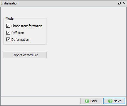
As the operation is added, Process settings page opens as shown in Fig. 3DHTWL1.4. User can set the simulation mode based on the simulation requirement along with step definition controls.

Turn on “Deformation “, “Diffusion “, and “PhaseTransformation “. Step definition will be defined in Simulation controls page. Click on leave the settings in initialization page as it is (see Fig. 3DHTWL1.5.) and click on .

Initialization Setup window

Material definition

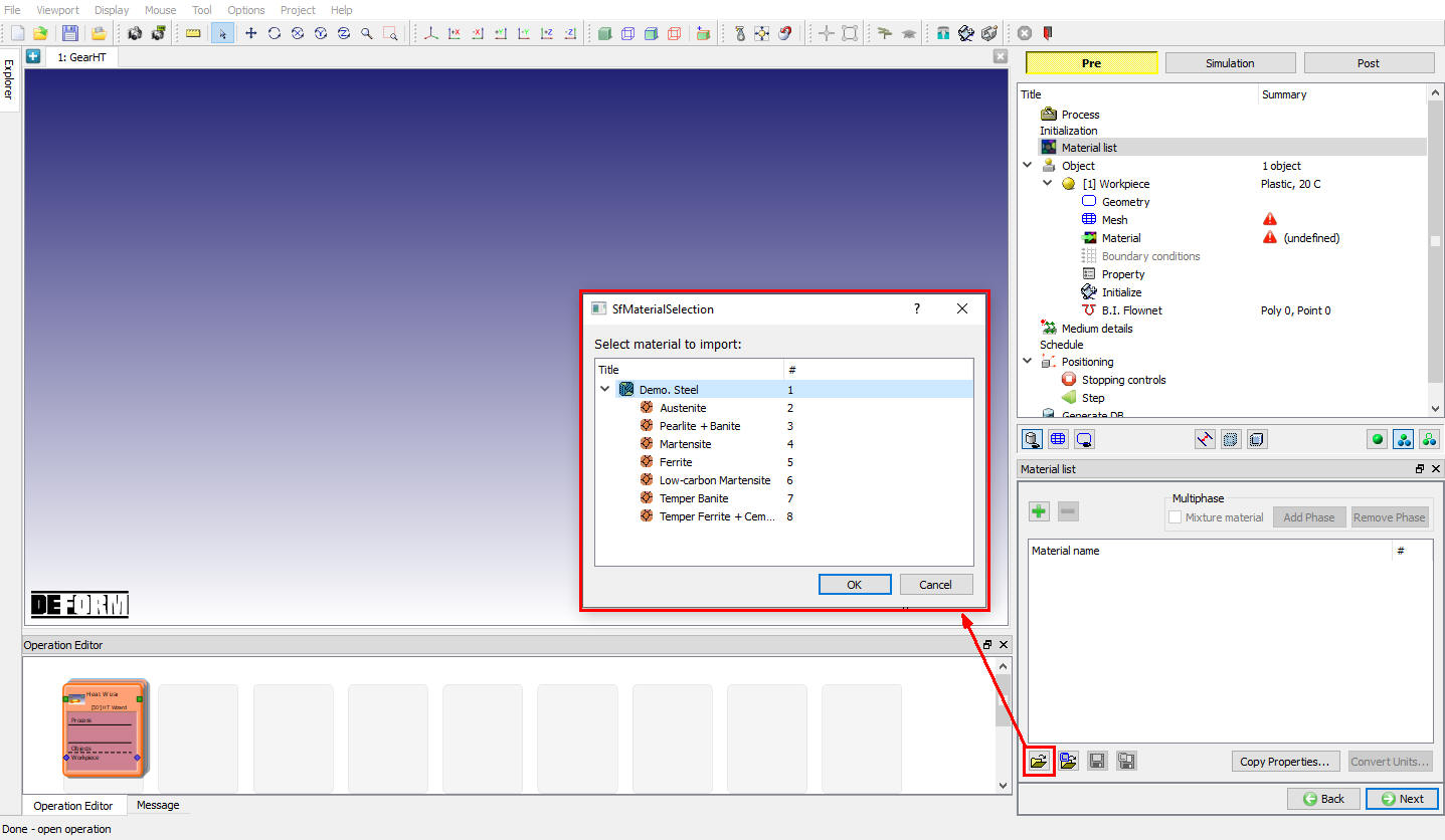
In Material page, click on (Import material from file) and import material “Demo_Temper_Steel.KEY “ from installation path \SFTC\DEFORM\v_\3d\LABS directory (see Fig. 3DHTWL1.6.). Click to material Selection popup dialog and click until workpiece object page.

Importing Material

Workpiece Object Type

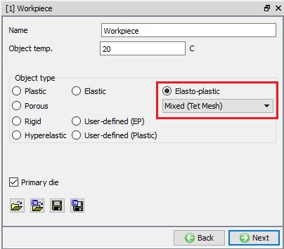
In Workpiece page, change the object type to Elasto-plastic type and select “Mixed (Tet mesh) “ as element type for Elasto-plastic from drop - down menu (see in Fig. 3DHTWL1.7.). Click to Geometry page.

Note : For almost all 3D heat treat models, (Tet Mesh) or brick mesh element should be used but not “Standard” tet.

Workpiece object page

Import Geometry

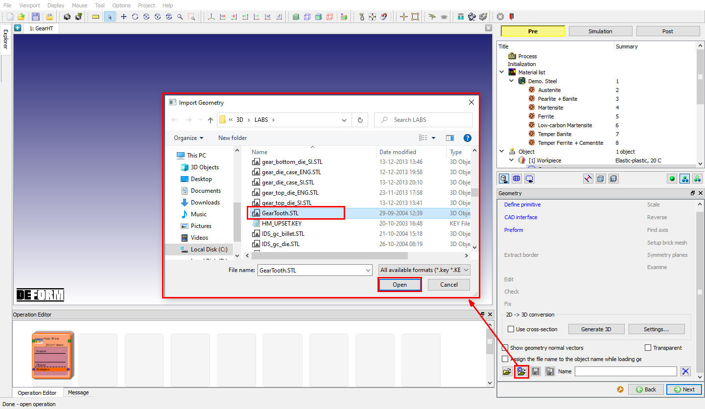
In Geometry page, click on (import geometry from library) option and import the GearTooth.STL file from installation path \SFTC\DEFORM\v_\3d\LABS as shown in Fig. 3DHTWL1.8. Use action label to check the Geometry. A perfect geometry should display message as shown in as shown in Fig. 3DHTWL1.9. Click .

Importing Geometry

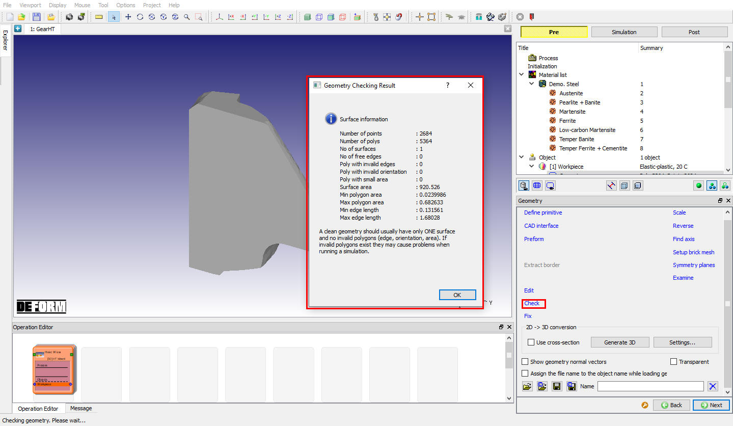
Check Geometry

Generate Mesh

In Mesh page, Enter Target number of mesh elements as 16000 or drag the slider bar to 16000 then click on . Mesh is generated and meshed object looks as shown in Fig. 3DHTWL1.10. Click .

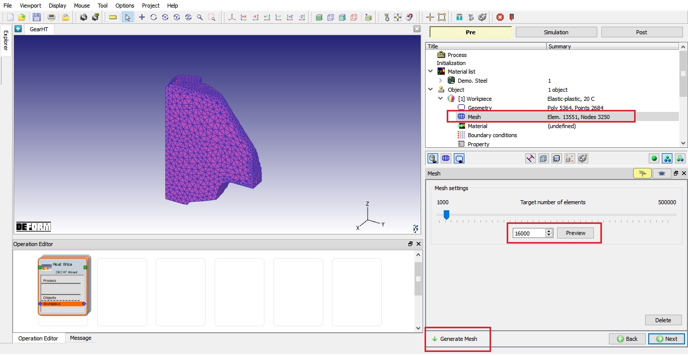
Generate Mesh Window

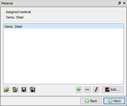
Assigning Material

Select and assign Demo.Steel Material as shown in Fig. 3DHTWL1.11. Click .

Assigning Material to workpiece

Assigning Boundary conditions

Assign symmetry surfaces on two sides of workpiece as shown in Fig. 3DHTWL1.12. Note that this geometry represents half a tooth of the gear.

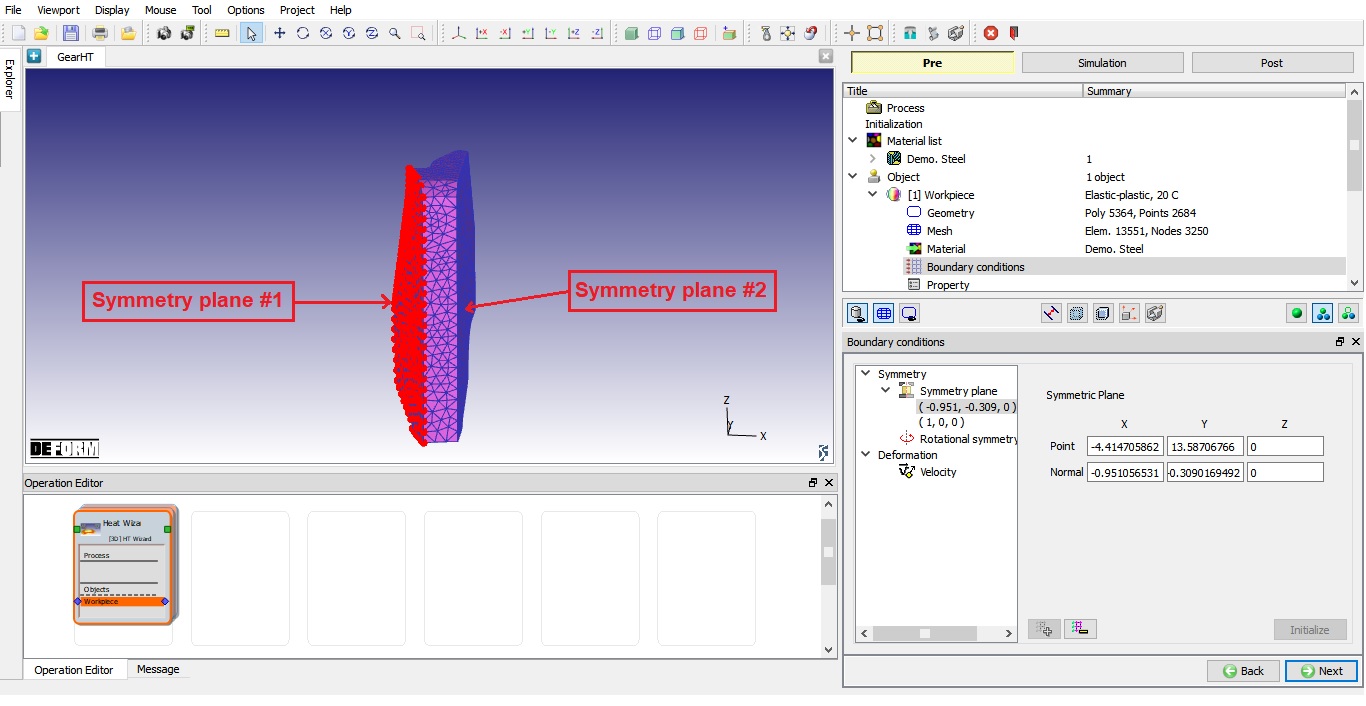
Assigning Symmetry BCC

In addition, as Elasto-plastic deformation will be modeled, some fixed-node boundary conditions need to be specified here. To do so, select a boundary condition item and then assign it to appropriate boundary nodes. For this model, as the symmetric planes provide the constraints in the directions perpendicular to their own plane, we need constraints in the Z direction. Here, we fix a node on the bottom as shown in the Fig. 3DHTWL1.13.

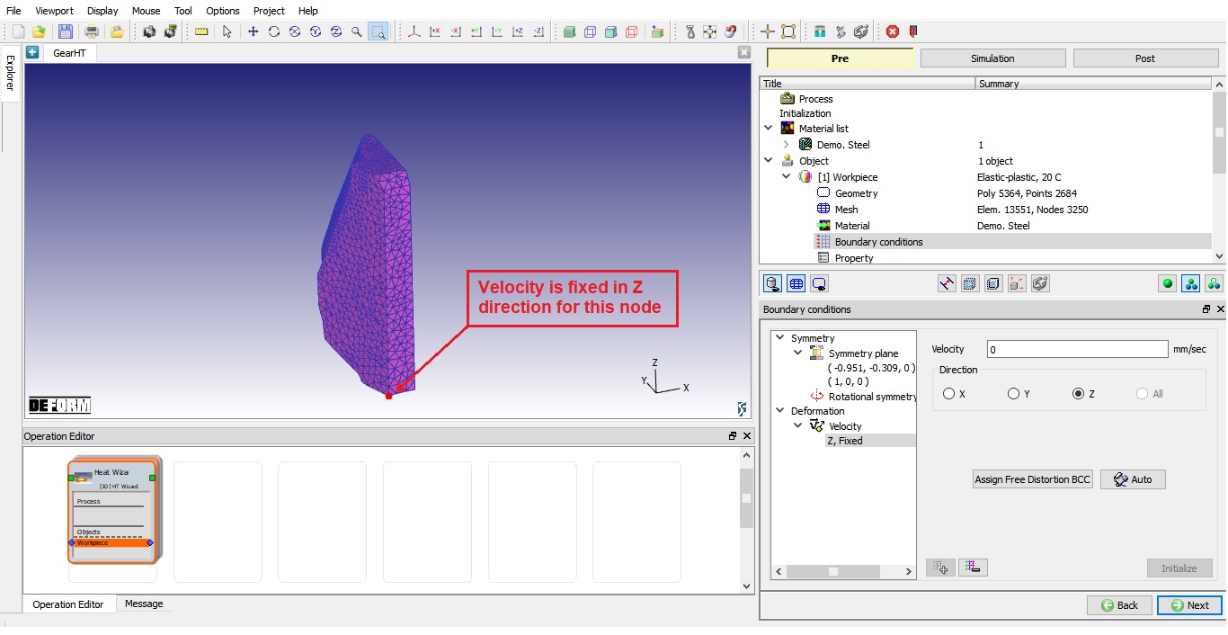
Assigning Velocity BCC

Workpiece initialization

Click on Object Nodes and select diffusion then define atompercentage as 0.2 using button (see Fig. 3DHTWL1.14.), assign using Range option by defining 0.2 as value then click on button. Click on button to close the Initialization dialog and click to close Nodal data dialog.

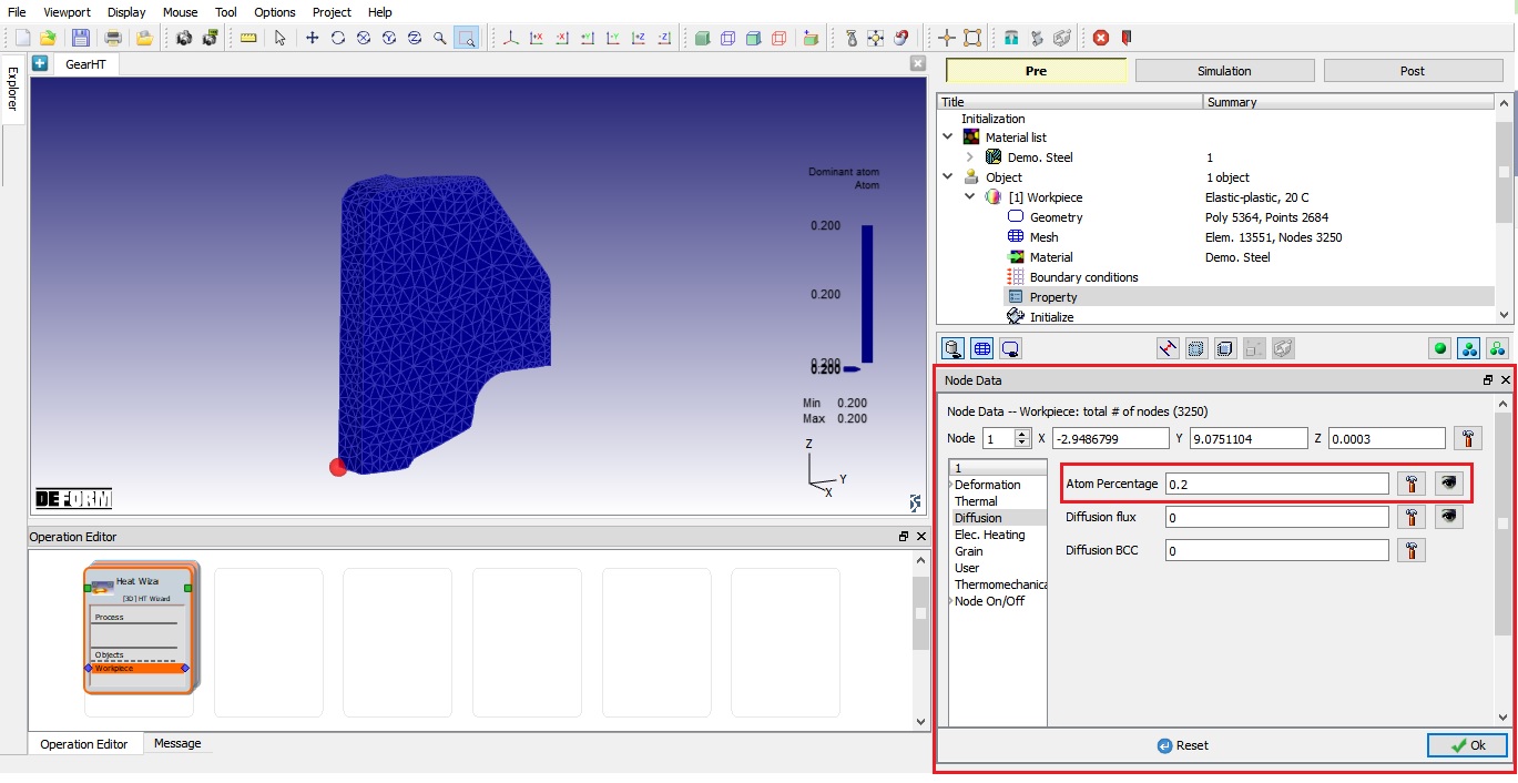
Object Node data definition window

Click on Object Elements and select Phasetransformation tab under Microstructure. Initialize Pearlite+Bainite as 1 and zero for the rest by selecting each phase and using (see Fig. 3DHTWL1.15.), assign using Range option by defining 1 as value then click on button. Click on button to close the Initialization dialog and click to close Element data dialog. Click to define the medium details.

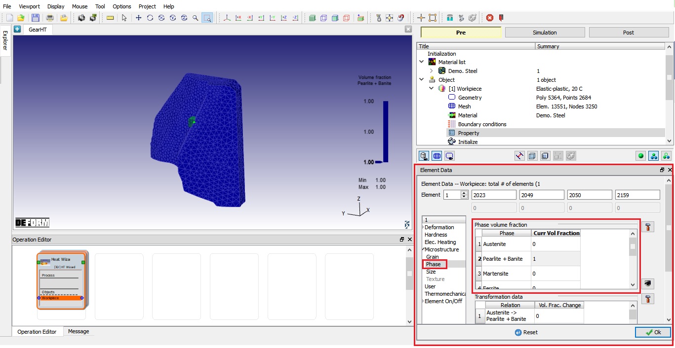
Object Element Data definition window

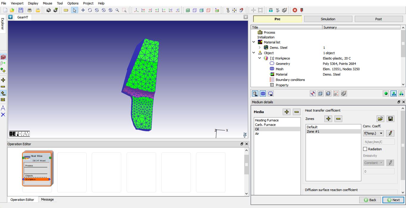
Medium Definition

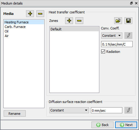
In page “Mediumdetails ”, you will define various media and heat transfer zones associated with them as shown in Fig. 3DHTWL1.16.

Medium Details window

Rename the first medium to “Heating Furnace” and set the “default” heat transfer coefficient (HTC) to constant 0.1. Activate Radiation by checking on Radiation button.
Add medium “Carb. Furnace” (Carb. for Carburization). Set the “default” heat transfer coefficient (HTC) to constant 0.05. For “Carb. Furnace”, input 0.0001 for the “Diffusion Surface Reaction Rate”. Activate Radiation by checking on Radiation button.
Add a media “Oil”. Deactivate the “Radiation”. Input 5.5 for the “default” HTC.

Add a heat transfer zone (Zone #1) to the media “Oil”. Click on the workpiece boundary to specify this zone to the bottom of the workpiece as shown in the Fig. 3DHTWL1.17. Note that you may need to change the picking modes in point selection window in order to specify the zone properly.

Medium detail window showing zone allocation

For Zone #1, define the HTC as a function of temperature as follows, by selecting f(Temp) from pull down menu and using button, (see Fig. 3DHTWL1.18. and Fig. 3DHTWL1.19. )

Temperature	HTC
20	2.1
250	2.8
500	6.8
750	4.0
1000	2.5

HTC table

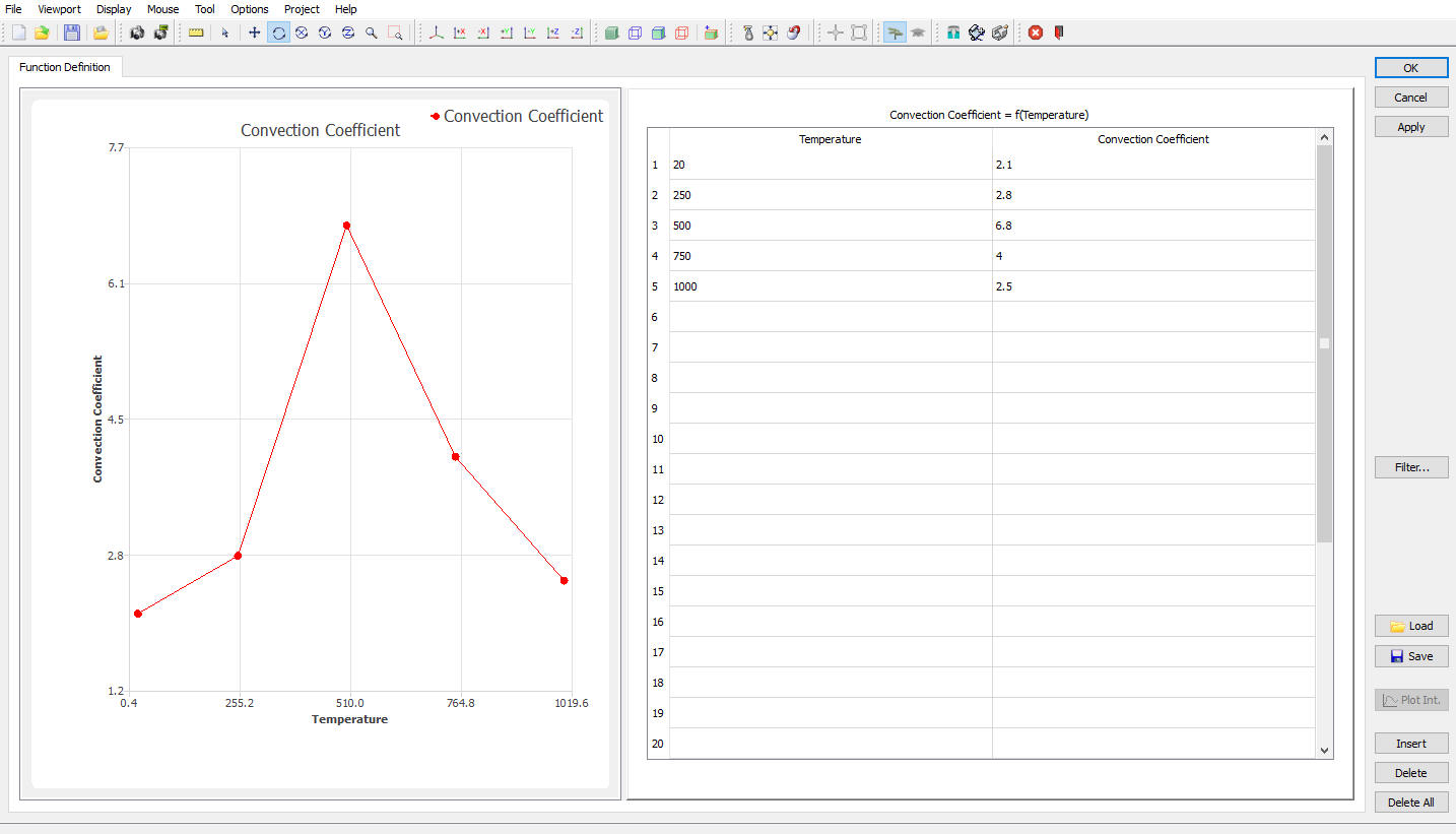
Function definition window

Add one more media “Air”. Input 0.02 for the default HTC. Activate Radiation by checking on Radiation button.

Scheduled Definition

In this lab we are going to carry out a five stage Heat Treatment process. In order to do this, in “Schedule” page, input a five-stage schedule as explained below.(See Fig. 3DHTWL1.20.)

Half an hour (1800 s) of pre-heating at 550C.
Two hours (7200 s) of carburization at 850C. Specify the “Atom” content to be 0.8.
20 minutes (1200 s) of oil quench with oil temperature 100C.
30 minutes (1800 s) of tempering at 280C.
One hour (3600 s) cooling in the air.

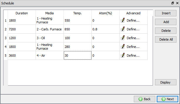
Heat Treatment Schedule window

The settings for each stage can be set or modified using button in advanced column. User can start from any stage by setting the Start Operation number based on the stages defined. For this lab we will use 1. Click on until Simulation controls page.

Simulation controls

In “Step Definition”, Select Auto radio button and change “Temp. Change per step” to 2 C. Accept other default settings. (See Fig. 3DHTWL1.21.)

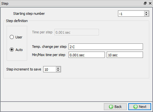
Simulation controls window

Generate Database

Click on action label to check the problem. Generate a database by clicking action label.

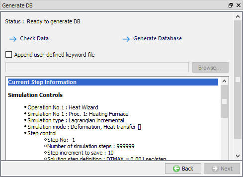
Generate Database Window

Starting the Simulation

Once the database has been generated, switch to the Simulation mode by clicking on button above the operation tree. Click on the action label to open the Run Options dialog as shown in Fig. 3DHTWL1.23. Use the default Continue Run option to select “Continue from the last step ” (from step -1) option and then select the Simulation mode as Interactive and click on button to run the simulation.

To define MPI settings, click on button, Run Options window will expand and displays options to define MPI settings for simulation (max number of processors that can be defined depend on your 3D MPI license).

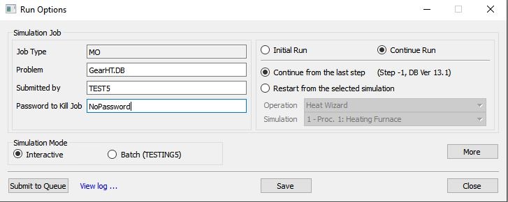
Run simulation window

The progress of the simulation can be monitored as it is running by looking at the Simulation Message and process monitor in Simulation mode. Click the Simulation Message tab to view the Message file. As long as the option is checked, which is the default setting, the Message file will refresh every couple of seconds.

The Message file provides information about which simulation step the simulation is currently on and also gives information dealing with how well the simulation is running.

When the simulation has finished, the message will be added to the end of the Message file. (See Fig. 3DHTWL1.24.).

Each stage defined will be executed as individual operation and user need to wait until all the stages simulation is completed.

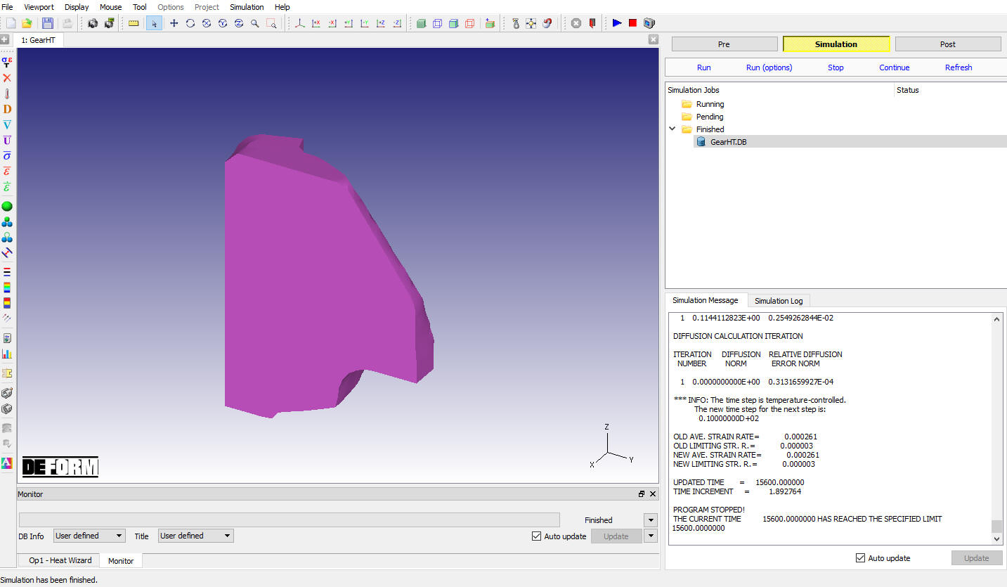
Simulation Message tab

Post processing

When the simulation has finished, click on . In Step Browser click on button to view all steps. The temperature min-max history should be like the graph below (see Fig. 3DHTWL1.25.).

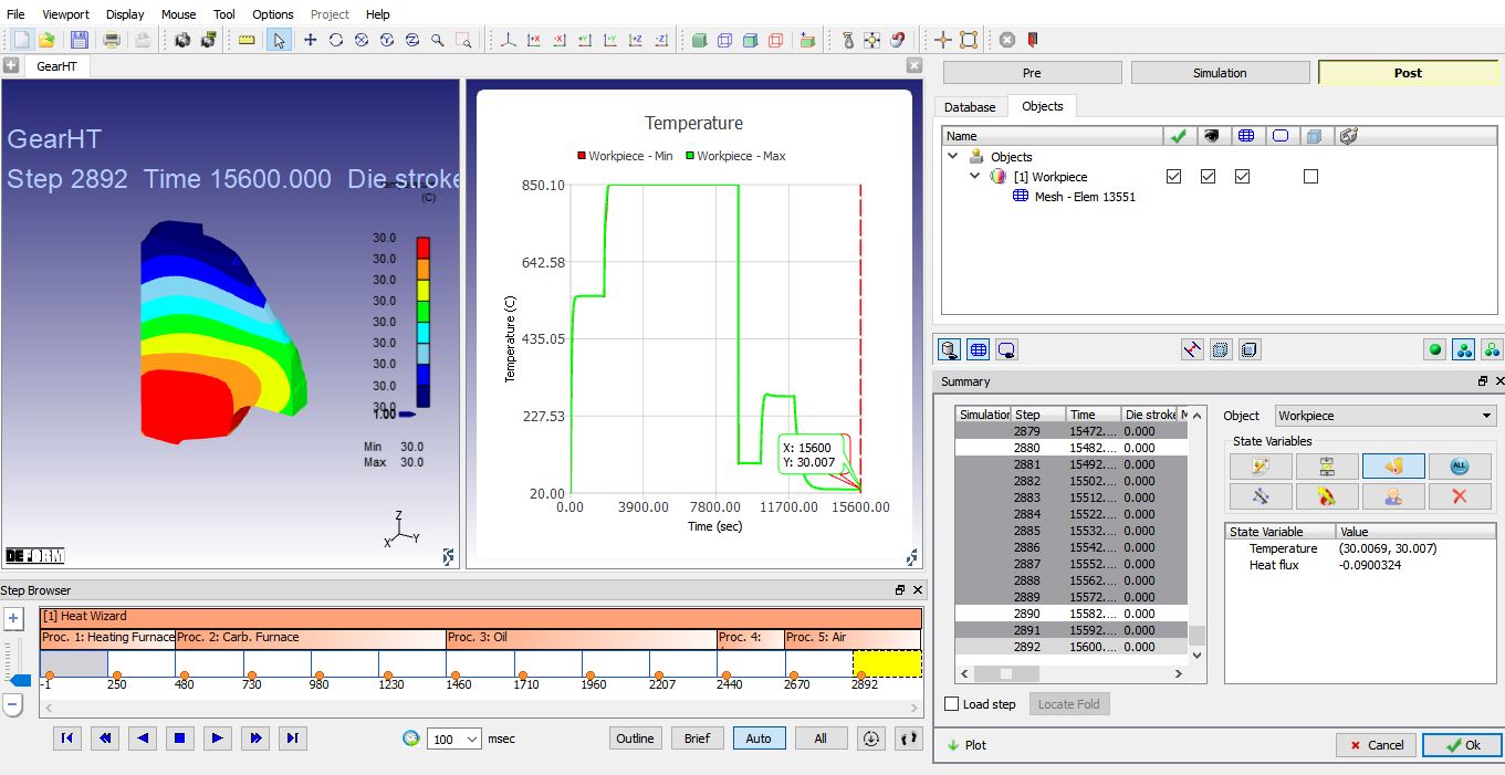
State Variable showing Temperature Min-Max history

In post-processing, we recommend following tasks to be performed:

Examine the state of the workpiece after oil quenching. The state variables of interest may include carbon content, volume fractions of Martensite (M), Ferrite (F), and Perlite + Banite (PB), and the residual stress. Note that at this point, M is as high as 0.797 near tooth surface, and the maximum effective stress is ~128 MPa.
Check the same state variables after tempering. Note that M is reduced to ~0.2 near tooth surface, most of which is transformed into Tempered Ferrite + Cementite (TFC). The maximum effective stress is reduced to ~82 MPa.
In addition, point tracking phase volume fractions at different locations of the work-piece can be helpful for understanding the complex phenomena occurred.