3D Cold Forming Lab

In this lab we will setup simple Bolt forming operation in MO 3D forming express operation. In this Forming operation we have 3 stages:

1. Extrude operation : In this operation, we are extruding the workpiece.

2. Cone blow operation: In this operation, we are upsetting the top side of the workpiece.

3. Hex Head operation: In this operation, we are giving Hexagonal shape to the top surface of the workpiece.

After completion of Forming operation, we will be doing Die stress to investigate stresses in the Top die.

Operation 1 : Extrude operation

Operation 2 : Cone blow Operation

Operation 3 : Hex head operation

Operation 4 : Die Stress Operation

Extrude operation

Creating a New problem

On a Windows machine , go to the button select DEFORM-v1x.xxx (.xxx indicates version number E.g. v14.0.2) and select DEFORM GUI Main vxx.xx from the menu. The DEFORM GUI Main window will appear, as shown in Fig. 3DCFL1.1.

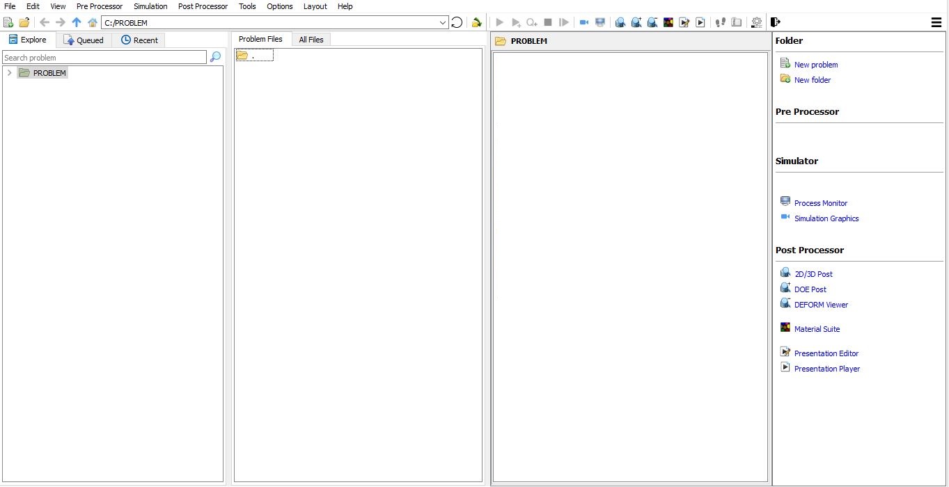
DEFORM GUI Main window

Create a new problem either by selecting File New Problem or by clicking the New Problem icon. The Problem Setup window will appear as shown in Fig. 3DCFL1.2. Select “Integrated Manufacturing Process “ radio button and unit system as “English “ radio button in unit field. Define Problem Name as “3D_**Bo lt ” and make sure the “Show option dialog” check box is turned on (if we do not turn on the “Show option dialog** ” check box, then we will not get the New Project dialog in MO UI). Then click on button to open a new Problem using the Deform Integrated Manufacturing Process.

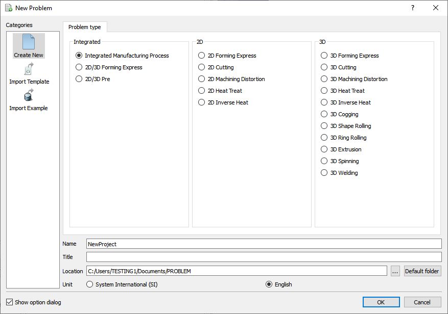
Problem type selection window

Multiple operation wizard will open with the New Project dialog (see Fig. 3DCFL1.3.), at this point user will be prompted to specify a project name (system will create a separate folder with this project name) and title for this session. In this session we will use “3D_**Bolt **” as the project name. Click on to continue to open the operation.

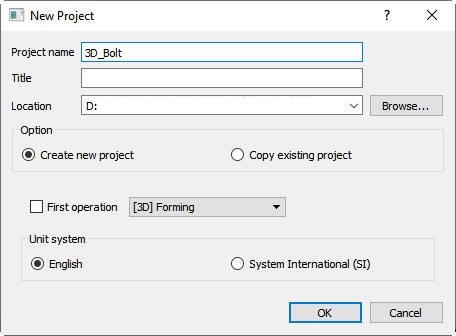
MO Wizard New Project

Add operations

Once you click on button, a Multiple Operation wizard will open to setup the problem. In this lab, we are showing how to setup all 3 operations in batch mode. Add three 3D Forming express operations from Operation list in Explorer. Operation can be added by clicking on button next to 3D Forming express operation or user can also add by drag and drop into the Operation Editor.

Change operation name:

Change the Operation name to “Extrude “ by double click on Forming field in Operation editor as shown in Fig. 3DCFL1.4.

Editing Operation name

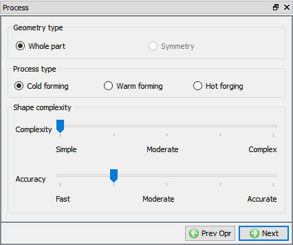
Define Process settings

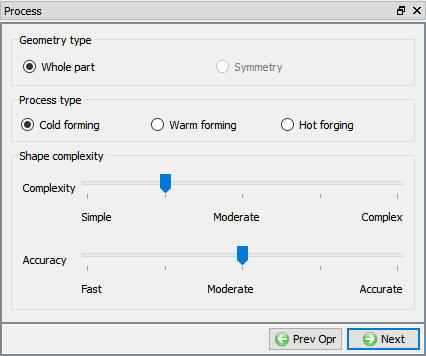
In Process page, select Process type as Cold Forming, select Whole part Geometry type.

The shape complexity and simulation accuracy slider bars influence the mesh settings and number of time steps used in the simulation. This in turn, influences the run time and level of details available in the simulation.

For this simulation, we will use complexity as Simple and Moderate accuracy, set the slider bars as shown in below Fig. 3DCFL1.5., click .

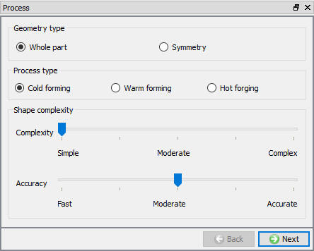
Process page

Adding Objects

In this operation we will use 1 workpiece + 2 dies as shown in Fig. 3DCFL1.6., click .

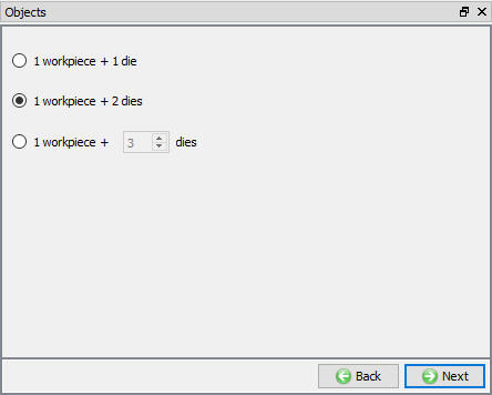
Number of Objects selection page

Workpiece Definition

Use default Workpiece object name and Default Object temperature, click .

Note : there is an button on the “Object” page. This is for importing complete object data from another DEFORM file, we will not use this at this time.

Import Workpiece Geometry

In Geometry page, click on Load Geometry from Library button, Import bolt-cutoff.STL file as shown in Fig. 3DCFL1.7.

Import object page

Click geometry. A description of what constitutes a legal geometry is given in the GEOMETRY CHECKING RESULT window as shown in Fig. 3DCFL1.8. The geometry of the bolt cutoff is legal. Then click .

Geometry checking page

Workpiece Mesh

Use the button to generate a surface mesh with the default number of elements. For the current settings used in Objects Shape Complexity, the default number of solid elements is 52000 as shown in Fig. 3DCFL1.9.

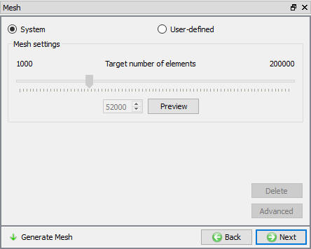
Mesh window in system mode

Go to Objects Shape Complexity and change Accuracy slider bar from Moderate to Fast. Go back to the Mesh screen and the mesh again. This time the default number of elements went down to 16,000. Similar results occur when changing the Accuracy slider bar.

Using advanced mesh generation

Select User defined radio button, Click on the button, select Min Element Size and enter an element size of 0.02” and use a Size ratio of 1 as shown in Fig. 3DCFL1.10. Click . The resulting surface mesh will be uniform with elements approximately .020”.

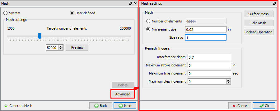
User defined Mesh advanced

Generate a mesh for use with simulations

The final mesh we generate will be used with subsequent simulations. Go back to Objects Shape Complexity, and change the slider bars back to Simple complexity and Moderate accuracy. Click on Mesh under Workpiece in the project tree, and then Generate mesh by clicking on ( will only generate a surface mesh while will create a surface mesh and then a solid mesh).

Assign Workpiece material

In Material window, load the material AISI-1010,COLD[70F(20C)] from DEFORM Material library, from Steel category using (Load material data from library) option. This can be done as shown in Fig. 3DCFL1.11. by clicking button. Material can also be loaded from Materials list in Explorer then click until Top Die page.

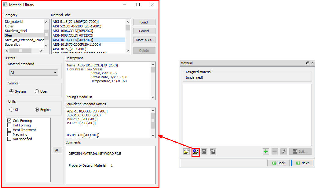
Material Library window

Top Die Definition

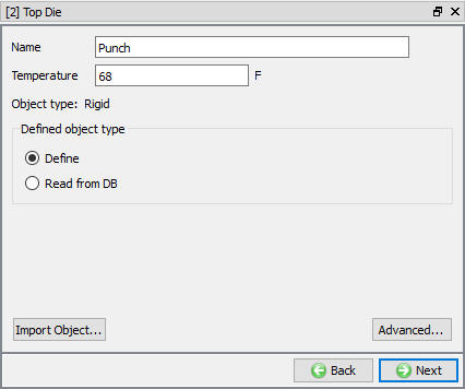
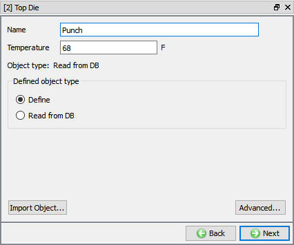
In Top Die page, change the object name as Punch and use the default Object Temperature (68F), click .

Import Top die geometry

Import bolt-punch1.STL file using Load Geometry from Library button as shown in Fig. 3DCFL1.12., then check the geometry using option. Click .

Importing Top die geometry

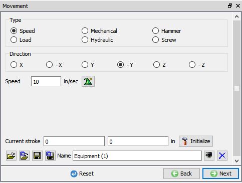
Assign Movement for Punch

Select speed under the movement options. Be sure movement is in the –Y direction, enter a speed of 10 in/sec as shown in Fig. 3DCFL1.13. Click .

Punch movement page

Bottom Die Definition

In Bottom Die page, Use the default Object temperature (68F), Click .

Import Bottom Die Geometry

Click on Load Geometry from Library button, Import bolt-die1.STL file. Then check the geometry using option. Click .

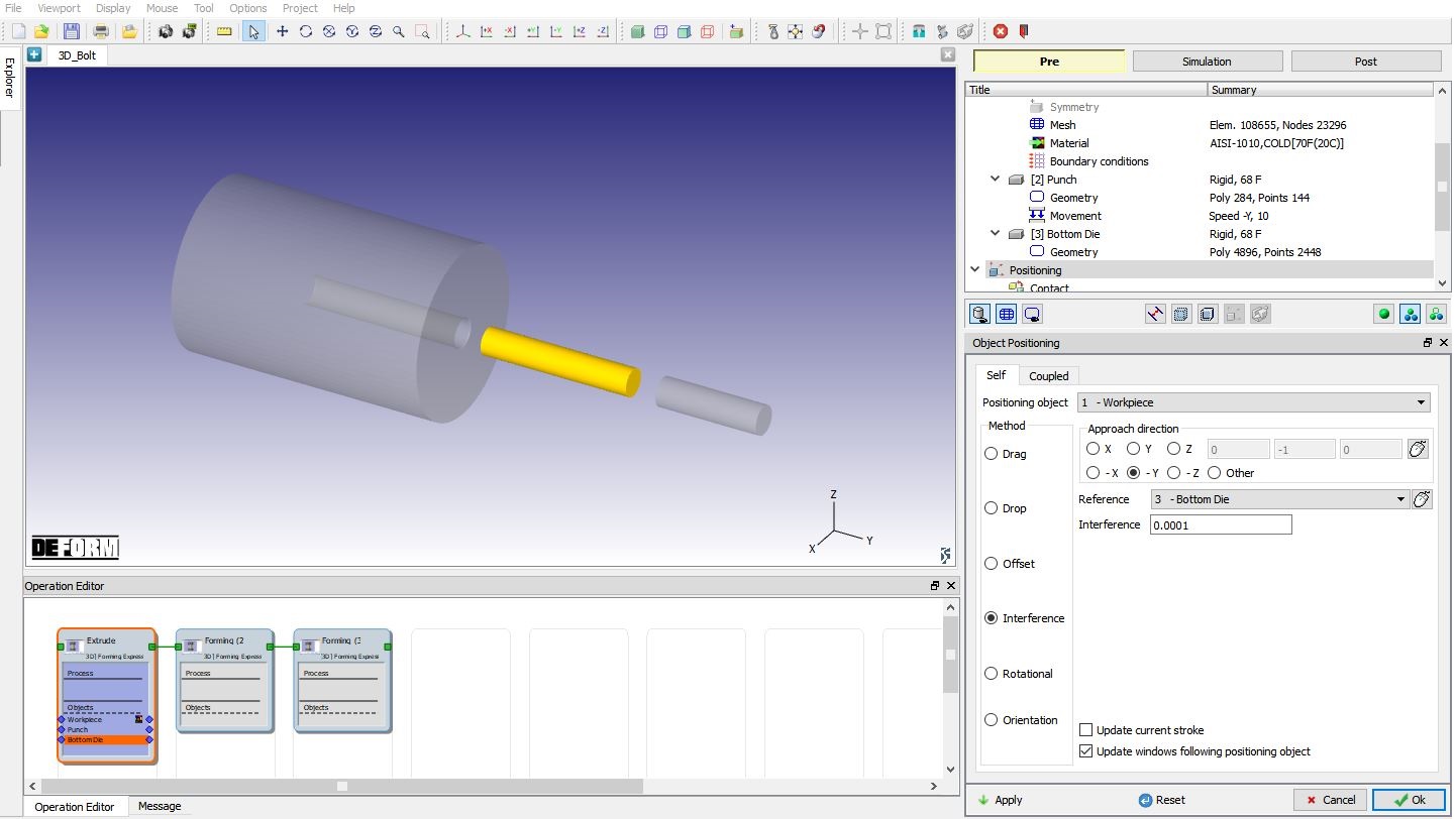
Objects Positioning

Click on button object positioning page will open, Select positioning and select Workpiece as Positioning object and Die as Reference. An approach direction of –Y should be used as shown in Fig. 3DCFL1.14., click . Similarly Position the Punch to contact the Workpiece using method with approach direction of –Y. The workpiece is positioned on the die and Punch is positioned on the Workpiece such that they are in contact with each other. Click .

Object positioning window

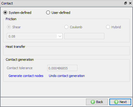
Define contact conditions

In the Contact section of the tree, by default the system defined default friction coefficient of 0.08 will be assigned, which corresponds to cold forming using carbide dies (see Fig. 3DCFL1.15.). By selecting User defined radio button user can also define other friction values if needed by using pull-down menu. DEFORM automatically determines an appropriate contact tolerance for this model. Click . You should be able to see the contacts between the Workpiece and other objects. Click .

Contact relation definition window

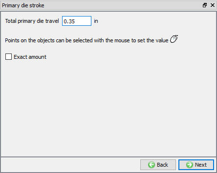
Assign primary die stroke

For this problem, we will extrude a distance of 0.35” as shown in Fig. 3DCFL1.16., so enter 0.35 “ in the Total primary die travel field then click .

Primary die travel definition window

Assign stop controls

We want to stop the simulation when the punch has moved 0.35”. Click Stopping Controls in the tree and check the Die stroke exceeds the value option. The value 0.35 ” defined in total primary die travel will be automatically placed in this field as shown in Fig. 3DCFL1.17. Click .

Stopping controls window

Review simulation controls

The number of simulation steps and the step increment are established by the Object Shape Complexity slider bar settings. If you want to change the default values, you can do by selecting user type radio button and define step definition. We will accept the default values for this lab.

Generate Database

In Generate DB page. Click the button to have the program check to see if anything was missed in the problem setup. During the checking process,

Messages in the red color signify data that needs to be fixed before a simulation can be run (such as when you forget to define any material data).

Click on button to generate the database. When the program is done writing the database, click on tab to go to Next operation.

Cone blow Operation

In this operation, we are importing new tools and changing Dies geometry.

Change operation name:

Change the Operation name to “Cone Blow “ in Operation editor as shown in Fig. 3DCFL1.18.

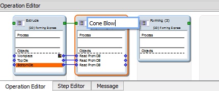
Changing operation name in Operation Editor

Define Process settings for Cone blow operation

Leave the Complexity as Simple and change the Accuracy to the tick mark between Fast and Moderate as shown in Fig. 3DCFL1.19. Click .

Process page

Adding objects

This operation will need one more object, so change the setting to 1 workpiece + 3 dies as shown in Fig. 3DCFL1.20., click until Top die page.

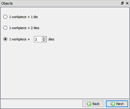
Number of Objects selection page

Top die Definition

In Object page, select Define radio button as shown in Fig. 3DCFL1.21. and change the object name as Punch , click .

Top Die page

Import Punch geometry

Click on Load Geometry from Library button, Importbolt-punch2.STL file. Then check the geometry using option. Click .

Define Punch movement

Use the previous operation’s movement data, Click .

Bottom Die Definition

In Object page, select Define radio button, click .

Import Bottom die geometry

Click on Load Geometry from Library button, Import bolt-die2.STL file. Then check the geometry using option. Click .

Ejector Definition

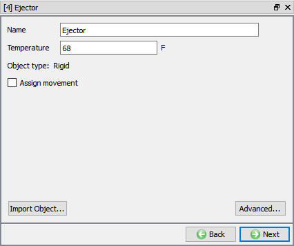
Change the Object 4 name to Ejector , then click .

Ejector page

Import Ejector die geometry

Click on Load Geometry from Library button, Import bolt-ejector2.STL file. Then check the geometry using option. Click unitl Scheduled positioning page.

Scheduled positioning

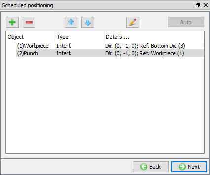
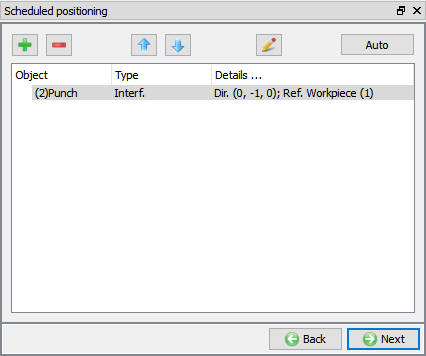
Using Interference positioning we will be positioning the Workpiece to the Die (-Y approach direction) and then the Punch to the Workpiece. In Scheduled positioning page, Click on button and select radio button. Change the Positioning Object to Workpiece and the Reference to Bottom di e. Change the Approach Direction to -Y and then click . Similarly, add interference scheduled positioning for Punch and Workpiece (-Y Approach direction for punch) as shown in Fig. 3DCFL1.23. Then click until Primary die stroke page.

Scheduled positioning window

Primary die stroke

We need to set the approximate amount the punch will move during this operation. the dies are around 0.8” apart in this operation. We want the punch and the die to be 0.25” apart at the end of the operation, so change this value to 0.6” as shown in Fig. 3DCFL1.24. Click .

Primary die stroke

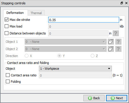
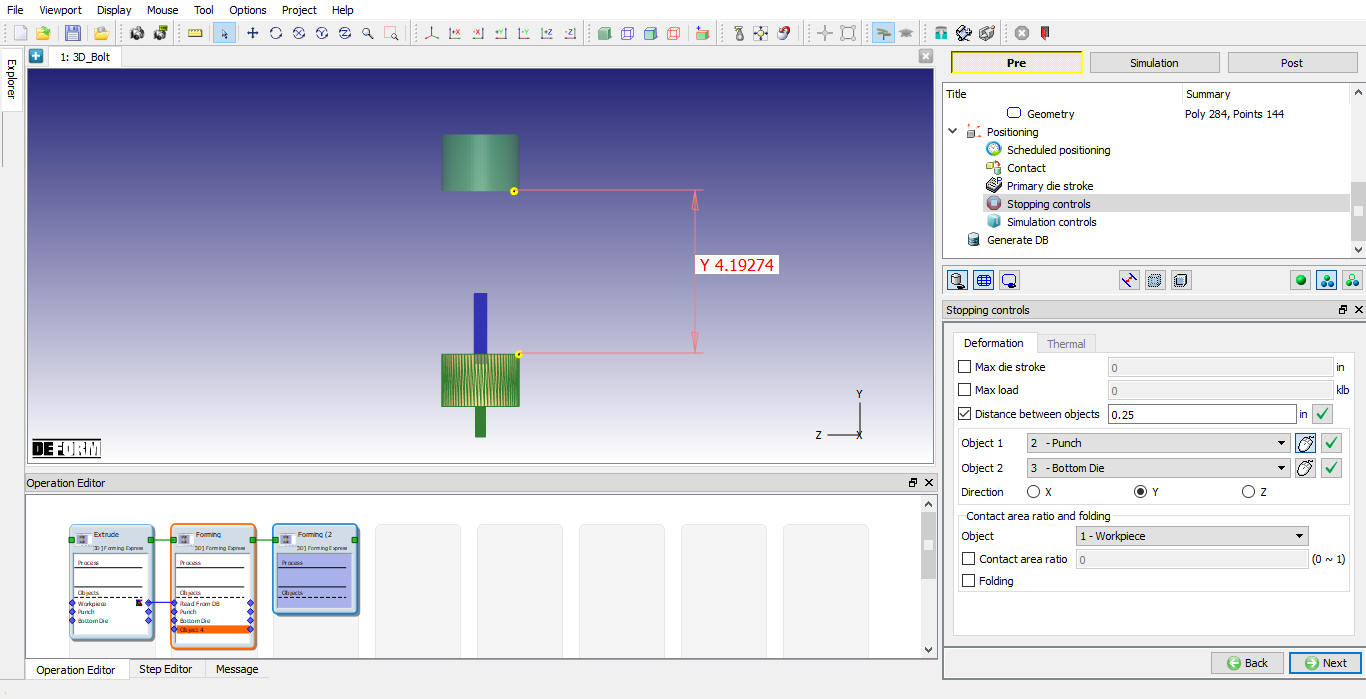
We want to form the part until the punch and die are within 0.25” of one another. In the Stopping Controls screen, place a check mark next toDistance between objects reaches to activate this option. With the mouse, click a point on the bottom of the punch and then click a point on the top of the die. An arrow between these two points should get displayed on the screen. Set the value for this distance to 0.25 ” in the Y direction as shown in Fig. 3DCFL1.25. Click .

Stopping controls window

Review simulation controls

The number of simulation steps and the step increment are established by the Object Shape Complexity slider bar settings. If you want to change the default values, you can do by selecting user type radio button and define step definition. We will accept the default values for this lab. Click .

Generate Database

See the Status in Generate DB page, if we see Input error, check the data missing and complete it. For this lab sequence expect “DB generation is not required for this operation. It will occur at run time.” message. Click on tab to go to Next operation.

Hex head operation

Change operation name:

Change the Operation name to “Hex Head “ in Operation editor.

Process Settings Definition

Change the Complexity to the tick mark between “Simple” and “Moderate” and increase the accuracy to “Moderate” as shown in Fig. 3DCFL1.26. Click until Top die page.

Process settings window

Top die Definition

In Object page, select Define radio button as shown in Fig. 3DCFL1.27. and change the object name as Punch , click .

Top Die general definition window

Import Punch geometry

Click on Load Geometry from Library button, Import bolt-punch3.STL file. Then check the geometry using option. Click .

Define Punch movement

Use the previous operation’s movement data, click on until Scheduled positioning page.

Scheduled positioning

Click on button and select radio button. Change the Positioning Object to the Punch and the Reference to the Workpiece and -Y approach direction, then click (see Fig. 3DCFL1.28.). Click on until Primary die stroke page.

Scheduled positioning window

Primary die travel Definition

In Primary die travel page, define primary die travel value as 0.4466 in as shown in Fig. 3DCFL1.29. Click .

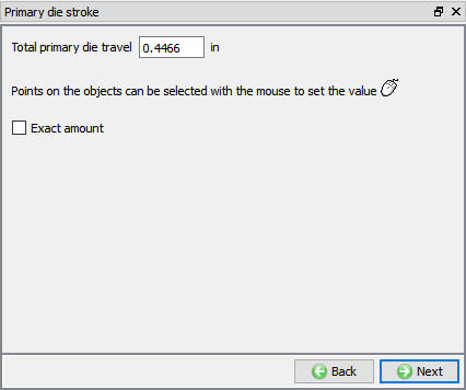
Primary die travel window

Stopping controls Definition

We want to form the part until the punch and die are within 0.03” of one another. In the Stop Controls screen, click “Distancebetween objects reaches ” to activate this option and set this to 0.03 ” in the Y direction. Click a point on the bottom of the punch and then click a point on the top of the die as shown in Fig. 3DCFL1.30. Click .

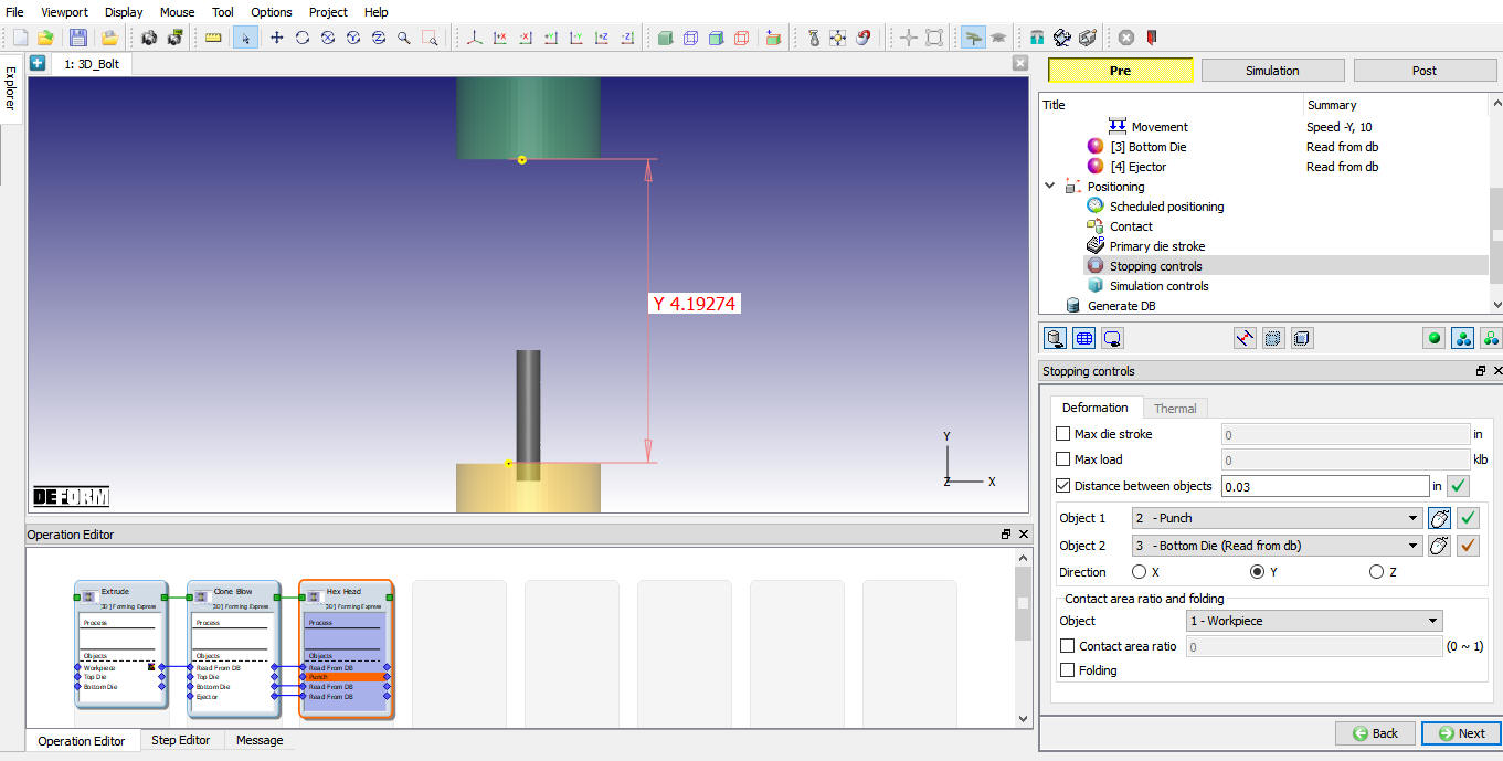
Stopping controls window

Review simulation controls

The number of simulation steps and the step increment are established by the Object Shape Complexity slider bar settings. We will accept the default values for this lab. Click .

Generate Database

See the Status in Generate DB page, if we see Input error, check the data missing and complete it. For this lab sequence expect “DB generation is not required for this operation. It will occur at run time.” message.

Save the project and click on mode to run the simulation.

Running simulation

Click on the action label to open the Run Options dialog as shown in Fig. 3DCFL1.31. Use the default Continue Run option to select “Continue from the last step ” option and then select the Simulation mode as Interactive and click on button to run the simulation.

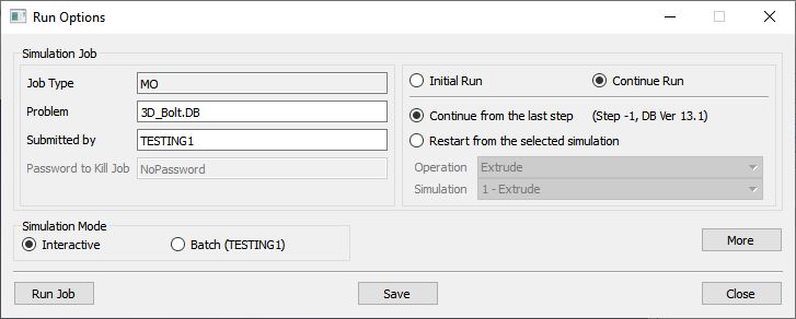
Run Simulation window

The progress of the simulation can be monitored as it is running by looking at the Simulation Message tab and Simulation Graphics from the Graphics display region in Simulation mode. As long as the option is checked in Simulation Message tab, which is the default setting, the Message file will refresh automatically.

The Message file provides information about which simulation step the simulation is currently on and also gives information dealing with how well the simulation is running.

When the simulation is finished without any issues, check the messages in LOG file, when all operation completes we will see in messages in LOG file:”MULTIPLE OPERATION COMPLETED “. (See Fig. 3DCFL1.32.)

LOG File

Postprocessing

After the completion of simulation, switch to mode. In Step Browser click on button to view all saved steps.

State variables:

From the State variables list, click the Effectivestrain icon to plot the amount of strain that went into the workpiece. To change the plot settings, you can click on the Set up icon. In this screen, you can display different kinds of contours (line, shaded or solid) as well as change the variable range that is shown on the contour bar (see Fig. 3DCFL1.33.). Using the Settings option, the range of the contour bar can be user-defined. Feel free to experiment with the display of the different state variables and plot options.

Strain Effective state variable plot

Slicing:

Use the Slicing tool to slice the workpiece and dies. State variables can be displayed on the sliced surface and by adding a slicing plane using the button, you can use multiple slicing planes. (See Fig. 3DCFL1.34.)

The slider bar in the SLICING window allows you to dynamically move the slicing plane.

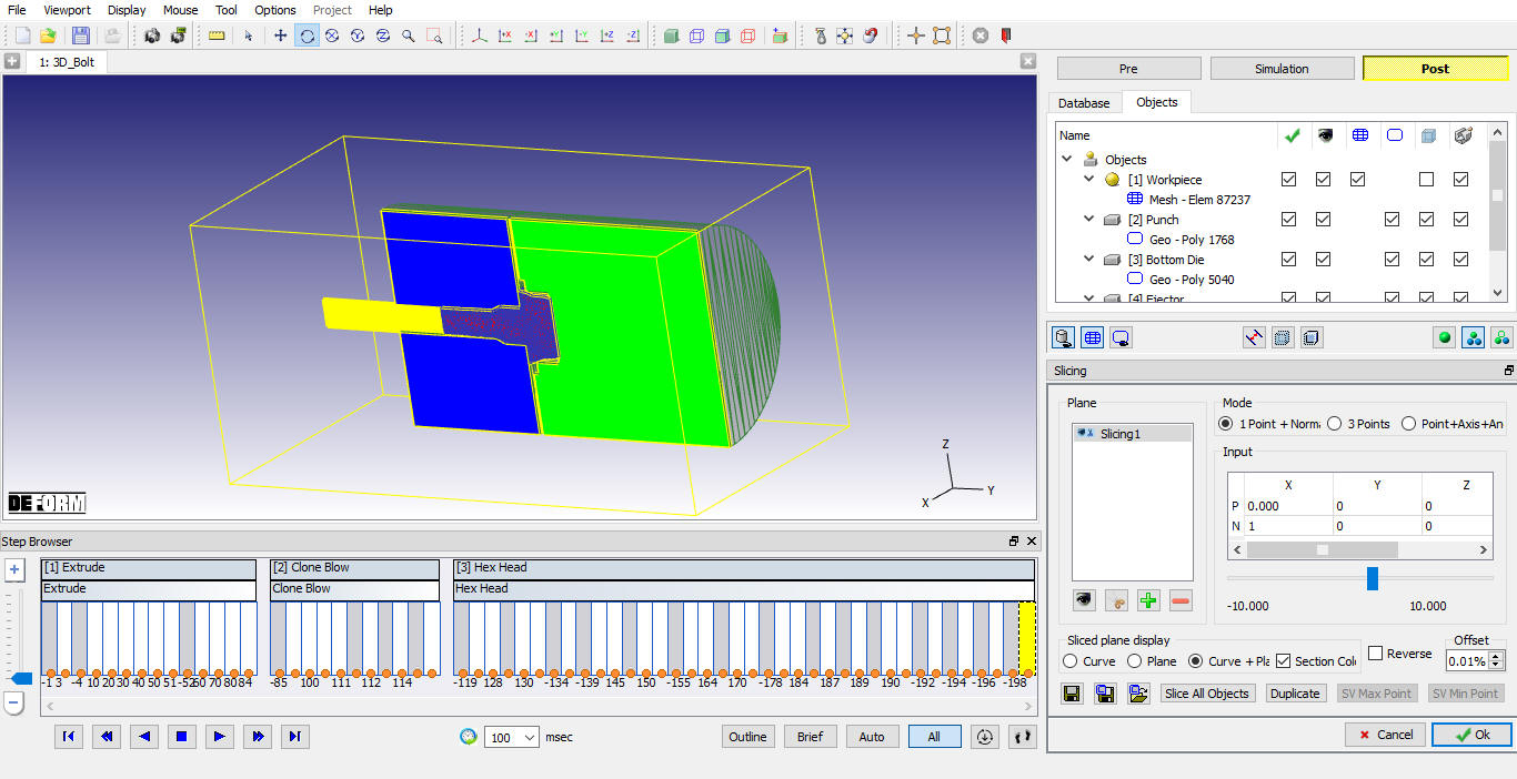
Slicing window

Point tracking:

Select Step –1 from the step list, and then select the Point tracking icon from the Tools list. Select few points on the object, and track the points. If a state variable such as effective strain is still being displayed, the values of the variable will be graphed at these points vs. time as shown in Fig. 3DCFL1.3.35.

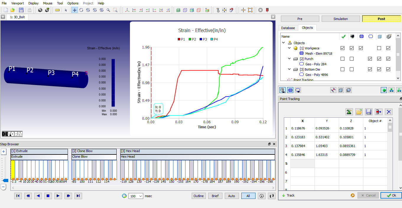
Point tracking graph plot

Load-Stroke:

The amount of load required to deform an object is an important result that can be obtained from a simulation. Click on the icon. When the GRAPH window appears, select only Punch in the object list, the X-Axis is set to Stroke and the Y-Axis is set to Y Load and select operation 3 for operation selection. Click and a Load-Stroke curve will display in the DISPLAY window as shown in Fig. 3DCFL1.36.

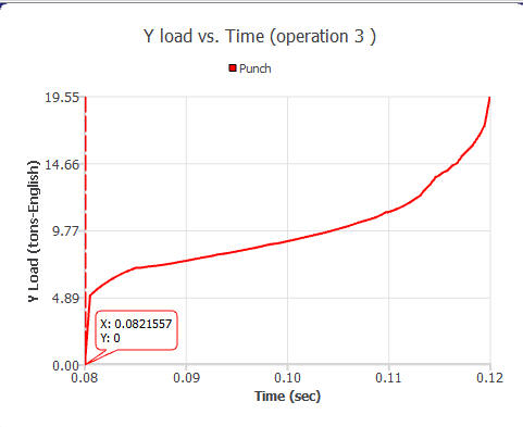
Load- stroke plot of Punch in Operation 3

Die Stress Operation

Add Die stress operation

After completion of Post process, switch to mode.

Add Die stress 3D operation from Explorer operation list, open added Die stress operation by double click on operation in operation list.

Select objects

We are currently only interested in the stress analysis of the punch in the hex head operation. So delete Bottom die (object3) and Ejector(object4) from the list by clicking delete button . Click . (See Fig. 3DCFL1.37.)

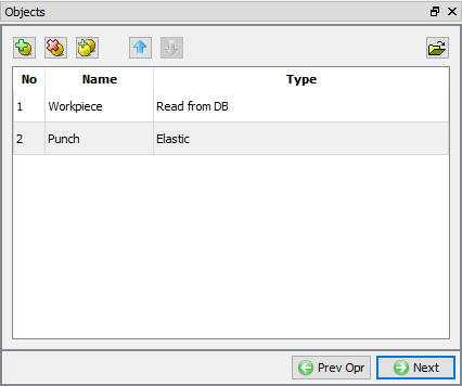
Die stress objects window

By default workpiece object type will be Read from DB, this object will be there upto DB generation, while generating DB it will be removed. Click .

Top Die Definition

By default Elastic radio button will be selected for top die then click to Mesh page.

Top die mesh page:

Define number of elements as 50000 as shown in Fig. 3DCFL1.38. and Generate mesh, then click until material page.

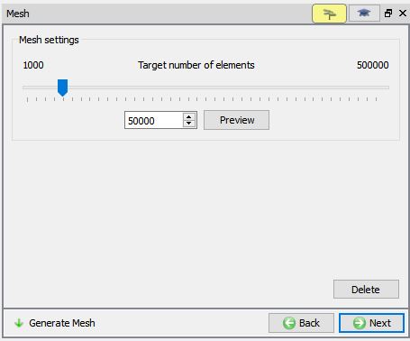
Mesh window

Assign material for Top die:

Import a die material from the material library. Chose AISI-H-13 from the list. Click

Assign Boundary condition for Top Die:

Next we need to apply boundary conditions to the punch so that it does not fly off into space when the forming loads are applied to it.

In the “Deformation BCC” screen, select the “All” velocities to be fixed and then select the back surface of the punch (may require that you rotate the punch around).

Once you have selected this surface, all the nodes on the surface should be highlighted. These nodes are currently selected but the boundary condition hasn’t yet been applied. Click the icon to apply the boundary condition to that surface. (See Fig. 3DCFL1.39.) Then click to Force interpolation page.

Adding Velocity Boundary condition

Force interpolation:

Once the mesh is generated, the forming loads from the workpiece need to be interpolated onto the punch. Click on Interpolate Force , Once the forces are interpolated, message will be displayed comparing the forces from the workpiece to the new forces on the punch as shown in Fig. 3DCFL1.40. These forces should be relatively close to one another (typically within about 5%). Click unitl Generate DB page.

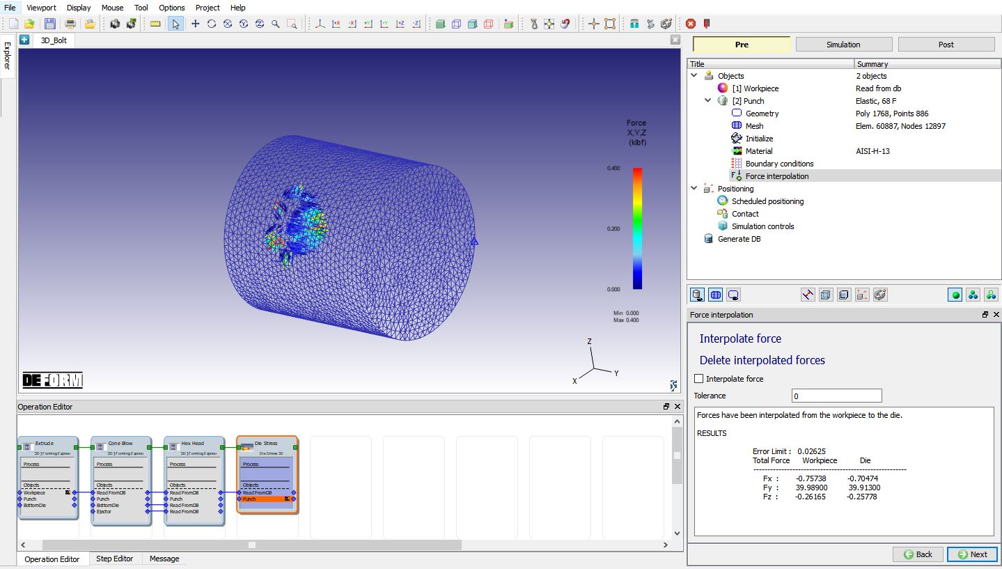
Force interpolation window

Generate DB

Check the data and generate the DB. After generating DB switch to mode to run the simulation.

Running simulation

Click on the action label to open the Run Options dialog. Use the default Continue Run option to select “Continue from the last step ” option and then select the Simulation mode as Interactive and click on button to run the simulation. As we click on button simulation starts.

After simulation is completed, switch to tab.

Post processor

The main variables to look at for a die stress simulation are the Effective stress and the Maximum principal stress.

The effective stress, is used to see whether any location in the die underwent plastic deformation. If any area of the die has an effective stress close to or exceeding the yield stress of the die material, that region is at risk of plastically deforming. (See Fig. 3DCFL1.41.)

The maximum principal stress is used to see which regions of the die are in a state of compression and which are in a state of tension. Maximum principal stress is extremely important in determining whether a die will experience any cracking due to fatigue. To display the maximum principal stress, click the state variable “Set up” button and then select Stress – Max Principal from the list. (See Fig. 3DCFL1.42.)

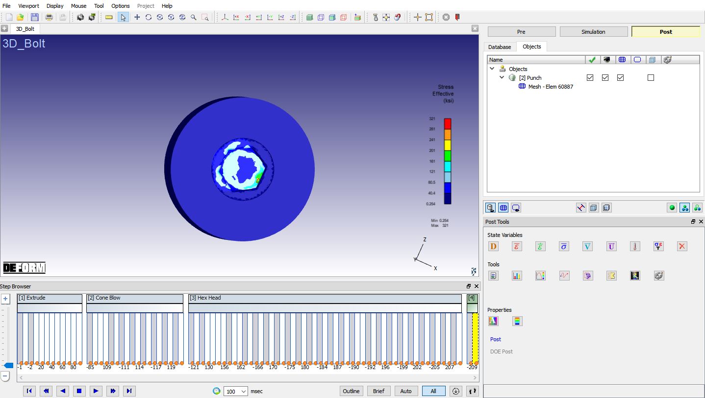
Stress-Effective plot

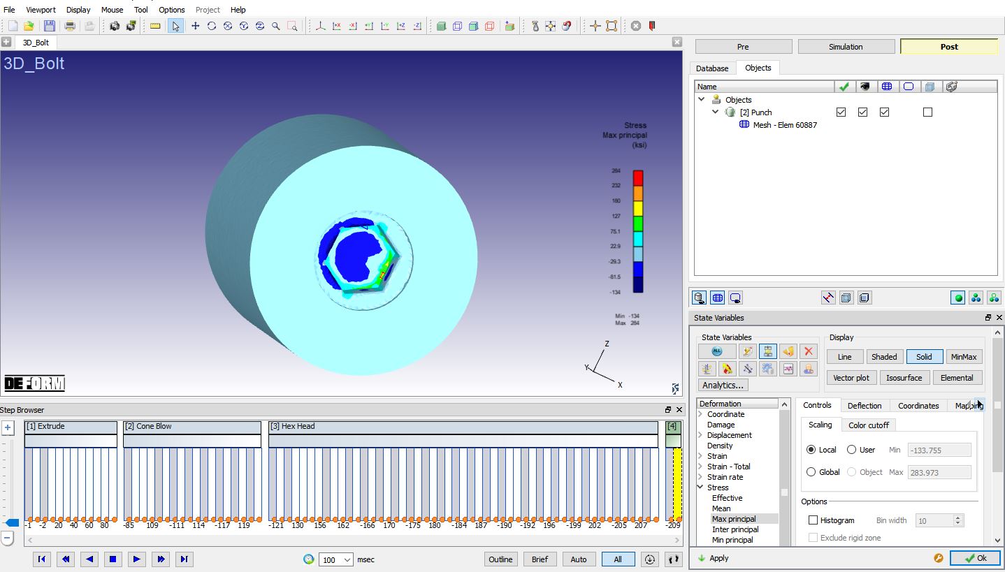
Max. Principal stress plot