51.1. 2D Inverse Heat Manual
51.1.1. How to open 2D Inverse Heat wizard
51.1.2. Initialization
51.1.3. Process condition
51.1.4. Material List
51.1.5. Workpiece object page
51.1.5.1. Geometry page
51.1.5.2. Mesh page
51.1.5.3. Material Page
51.1.5.4. BCC Page
51.1.5.5. Property Page
51.1.6. Temperature Measurement Points
51.1.7. Time Zones
51.1.8. HT Zone Partitioning
51.1.9. Heat Transfer Zones
51.1.10. Positioning
51.1.11. Step
51.1.12. Optimization Controls
51.1.13. Generate DB
51.1.14. Post-Processing the Inverse HT Optimized results
How to open 2D Inverse Heat wizard
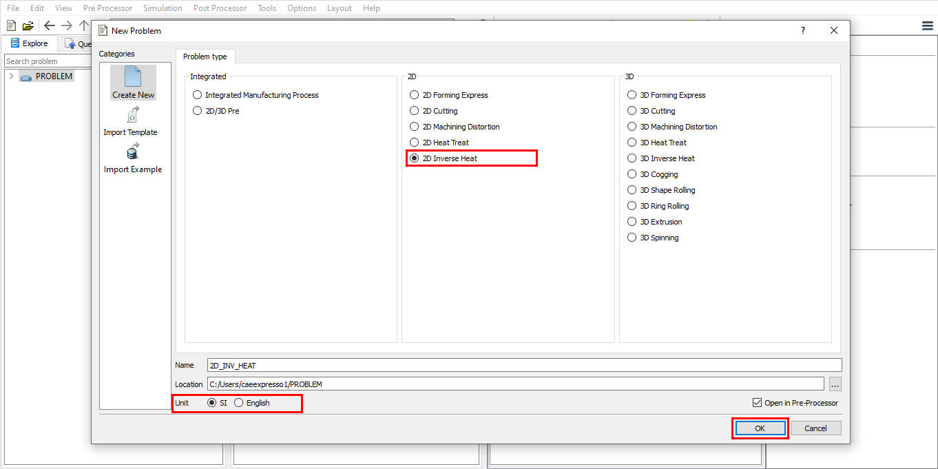
2D Inverse heat wizard can be accessed from GUI Main. Create a new problem by either selecting File![]() **New Problem** or by clicking the New Problem
**New Problem** or by clicking the New Problem ![]() icon. Select 2D Inverse heat Problem type and unit system as shown in the Fig. 51.1.1. then click
icon. Select 2D Inverse heat Problem type and unit system as shown in the Fig. 51.1.1. then click ![]() . 2D Inverse Heat Wizard will be opened and in Operation editor we can observe 2D Inverse heat operation being added as shown in Fig. 51.1.2.
. 2D Inverse Heat Wizard will be opened and in Operation editor we can observe 2D Inverse heat operation being added as shown in Fig. 51.1.2.
Opening 2D Inverse heat Wizard from GUI Main
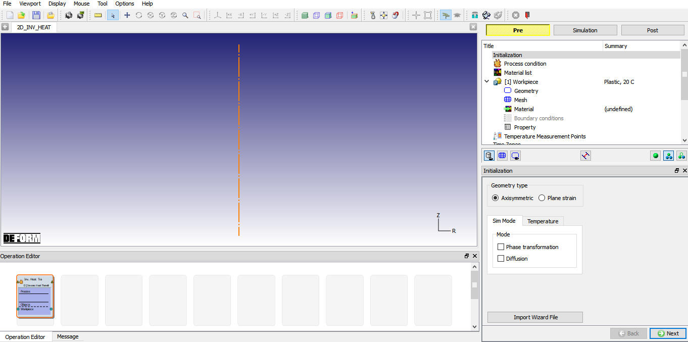
2D Inverse Heat Wizard
Initialization
The user can select the Geometry type and mode to continue the setup. In this page user have options to import wizard file using ![]() button, “*.IHWZ” file will be imported as shown in the Fig. 51.1.3. In Sim mode tab, depending on the requirement user can turn on the Phase transformation check box to include phase transformation calculations and Diffusion check box to include atom diffusion while estimating the Heat transfer Coefficients (HTC).
button, “*.IHWZ” file will be imported as shown in the Fig. 51.1.3. In Sim mode tab, depending on the requirement user can turn on the Phase transformation check box to include phase transformation calculations and Diffusion check box to include atom diffusion while estimating the Heat transfer Coefficients (HTC).
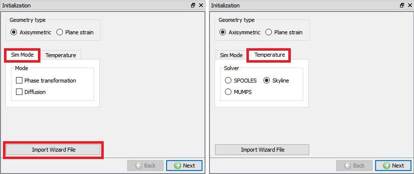
Initialization page
Process condition
In Inverse HT wizard user can model both heat transfer while transferring to quenching and then Quenching. Depending on the requirement user can select any one or both processes. Heat transfer operation will be simulated first followed by quenching. User need to define the environment temperature data for the selected process as shown in the Fig. 51.1.4. The environment temperature can be defined as a constant or function of time.
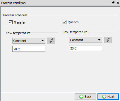
Process condition page
Material List
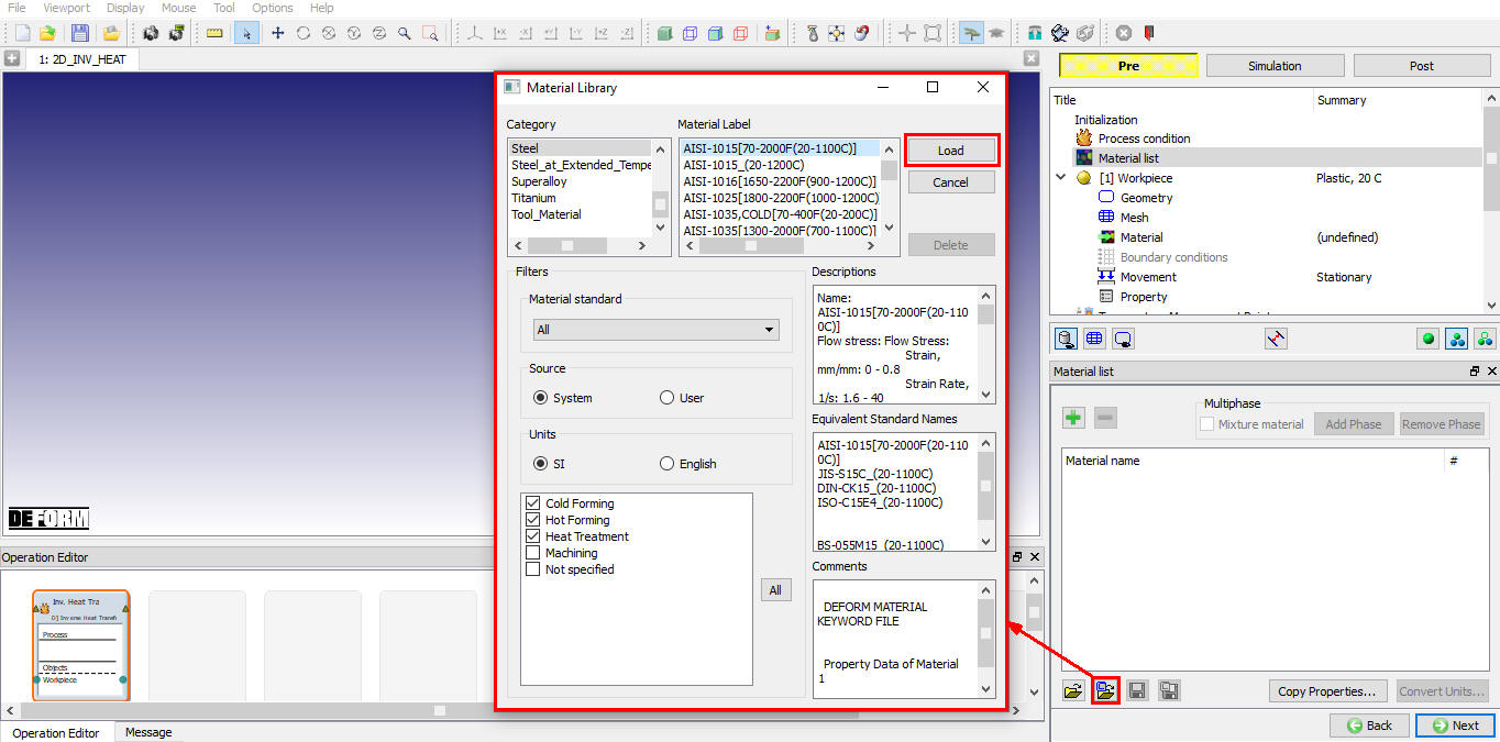
In this Material List page, user can load the material for the Workpiece using Import Material data from a File ![]() or using Load form Library option
or using Load form Library option ![]() . If user has created a new material, then user can save the material using
. If user has created a new material, then user can save the material using ![]() ,
, ![]() buttons. (See Fig. 51.1.5.)
buttons. (See Fig. 51.1.5.)
Material List Page
Workpiece object page
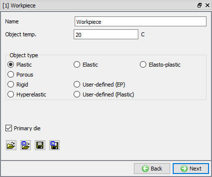
In Workpiece page, user can define object name, object initial temperature and object type of a workpiece as shown in the Fig. 51.1.6. The object type is selected as “Plastic” by default, if user is interested to consider the effect of elastic properties then Elasto-plastic object type can be used. User can import objects from other databases or key files using ![]() ,
, ![]() options or save the object data using
options or save the object data using ![]() ,
, ![]() options.
options.
Workpiece Object page
Geometry page
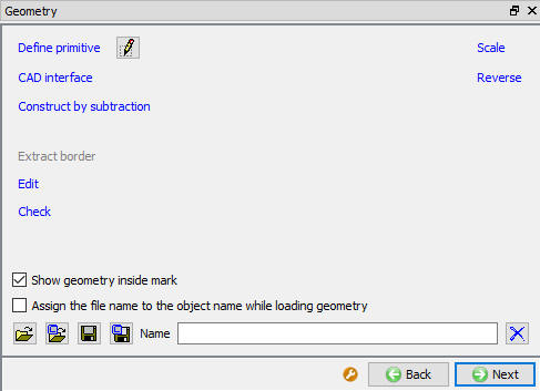
The geometry can be imported from a file using ![]() ,
, ![]() options or can be created from the primitives. Modifications to the imported or created geometry can be made using
options or can be created from the primitives. Modifications to the imported or created geometry can be made using ![]() option. The geometry can be saved using
option. The geometry can be saved using ![]() ,
, ![]() options. (See Fig. 51.1.7.)
options. (See Fig. 51.1.7.)
Geometry Page
Mesh page
Mesh Page provides options to mesh the object. Guided ![]() mode provides option only to set number of elements using slider bar to generate mesh. If the object geometry is complex or user would like to control the mesh density over the object, then user must switch to expert mode by clicking on
mode provides option only to set number of elements using slider bar to generate mesh. If the object geometry is complex or user would like to control the mesh density over the object, then user must switch to expert mode by clicking on ![]() . Expert mode provides various options like weighing factors and mesh windows and user defined mode to control the mesh density. Meshing options available in Guided mode and expert mode are shown in Fig. 51.1.8. and Fig. 51.1.9.
. Expert mode provides various options like weighing factors and mesh windows and user defined mode to control the mesh density. Meshing options available in Guided mode and expert mode are shown in Fig. 51.1.8. and Fig. 51.1.9.
For more detail description of these options, please refer 2D Mesh page.
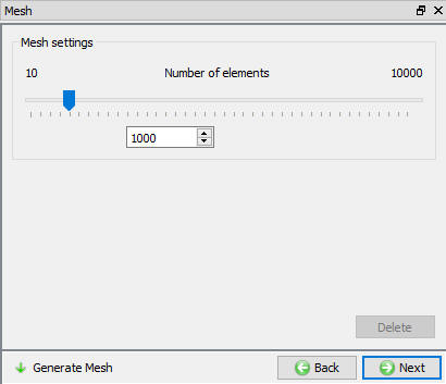
Guided Mode mesh options
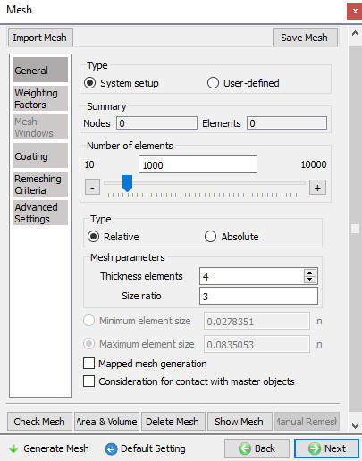
Expert Mode mesh options
Material Page
In material page, all the materials added to material list are displayed as shown in Fig. 51.1.10. User can select the required material to assign it to respective object. If the desired material is not available in the list, then the user can load the material in object material page using Import Material data from a file ![]() or using Load form Library option
or using Load form Library option ![]() . User can also create new material if the material is not available in DEFORM library using
. User can also create new material if the material is not available in DEFORM library using ![]() . User can delete the material from list using
. User can delete the material from list using ![]() or edit the material data using
or edit the material data using ![]() . Modified / newly defined Material can be saved using
. Modified / newly defined Material can be saved using ![]() ,
, ![]() .
.
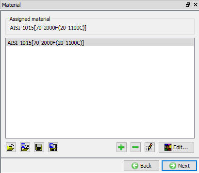
Assigning material to workpiece
BCC Page
In Boundary conditions page, user can assign various boundary constraints to an object. Boundary conditions specify how the boundary of an object interacts with the environment. Commonly used boundary conditions are heat exchange with the environment for simulations involving heat transfer and prescribed velocity for enforcing symmetry. (See Fig. 51.1.11.)
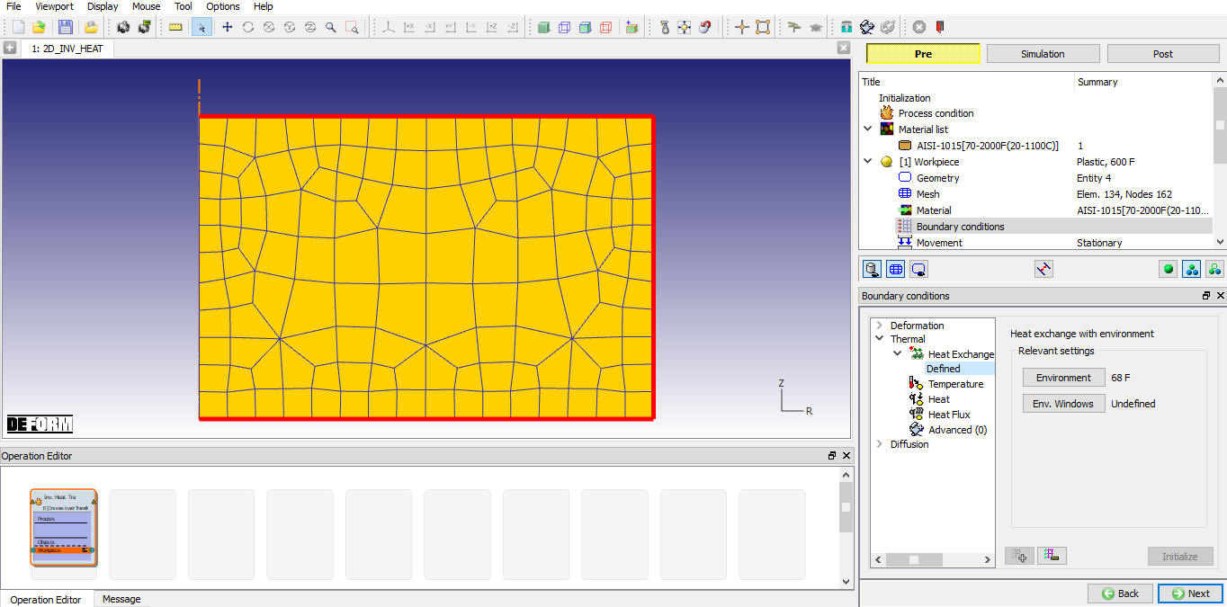
BCC Page
Property Page
Miscellaneous object parameters, which affect either thermo-mechanical behaviour of the object or numerical solution behaviour are specified in the Object-Properties window (See Fig. 51.1.12.). For more information please refer Object properties.
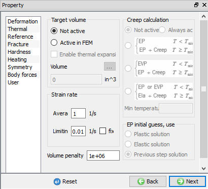
Property Page
Temperature Measurement Points
The user can define the temperature measurement points by clicking on add button and selecting the point on the workpiece as shown in the Fig. 51.1.13. The user can define the thermal data measured from experiments for the respective point using ![]() button as shown in the Fig. 51.1.14. or we can import the .DAT file containing the thermal data using the
button as shown in the Fig. 51.1.14. or we can import the .DAT file containing the thermal data using the ![]() option. We can also save the defined thermal data using the
option. We can also save the defined thermal data using the ![]() button. After defining the thermal data, the
button. After defining the thermal data, the ![]() button will change to
button will change to![]() button.
button.
The ![]() button is used to display experimental temperature curves at all points as shown in the Fig. 51.1.15. User can plot the temperature curves selectively by turning on or off the respective measurement points check boxes, “Hide All” and “Select All” buttons can be used to hide or display curves at all measurement points respectively.
button is used to display experimental temperature curves at all points as shown in the Fig. 51.1.15. User can plot the temperature curves selectively by turning on or off the respective measurement points check boxes, “Hide All” and “Select All” buttons can be used to hide or display curves at all measurement points respectively.
The temperature curves defined from experiments can have large number of values and user can filter the data by applying the tolerance value and using either “Collinear points” or “Douglas-Peucker” method. After defining the tolerance value and selecting the method of filtering, user can click on ![]() button to observe the effect of tolerance value and use “Reset” button to go back to previous experimental data before entering the filtering window. User can apply filtering to the selected curves using “Selected Curve only” check box.
button to observe the effect of tolerance value and use “Reset” button to go back to previous experimental data before entering the filtering window. User can apply filtering to the selected curves using “Selected Curve only” check box.
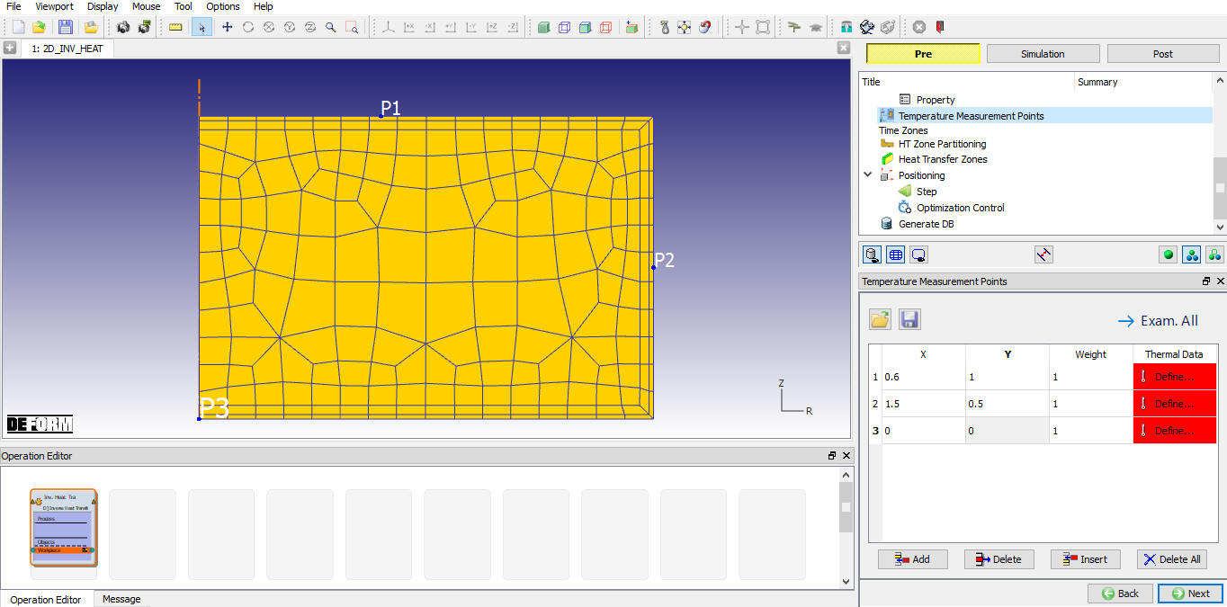
Temperature Measurement Points Page
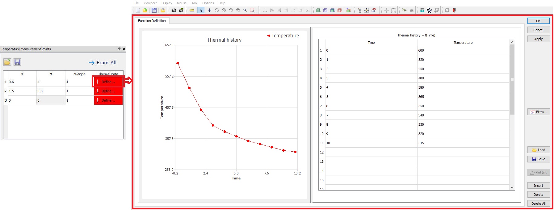
Defining the Thermal Data by using Define button
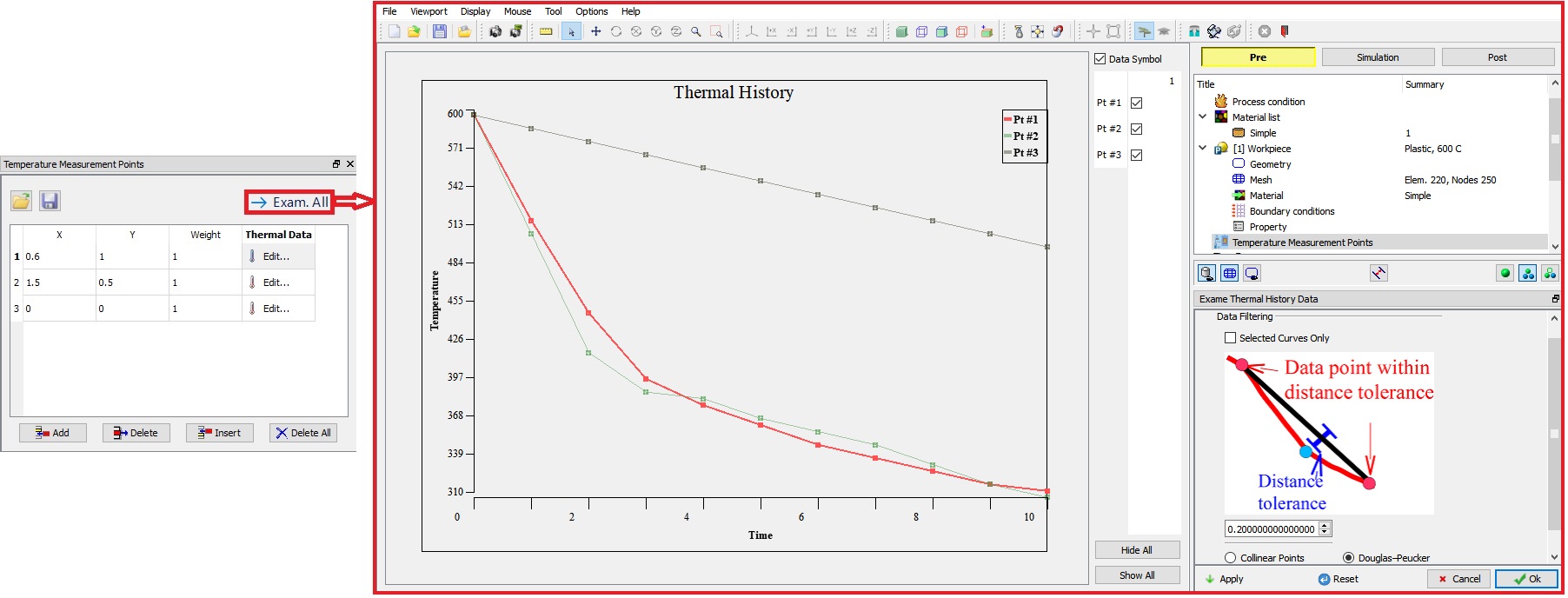
Display of all points thermal data using Exam all button
Time Zones
Time zone page provides option to define the duration of the selected processes in “Process Condition” page. If user has selected both processes, then “End time” of the “Transfer” process is automatically assigned to the “Start time” of the Quench, see Fig. 51.1.16. and Fig. 51.1.17. If user clicks on ![]() button without defining any data, then “End time” will be assigned as 10 secs. Display area displays the graph with temperature curves of all measurement points, a vertical line can be observed when both the processes are used indicating the end of “Transfer” process and start of “Quench”.
button without defining any data, then “End time” will be assigned as 10 secs. Display area displays the graph with temperature curves of all measurement points, a vertical line can be observed when both the processes are used indicating the end of “Transfer” process and start of “Quench”.
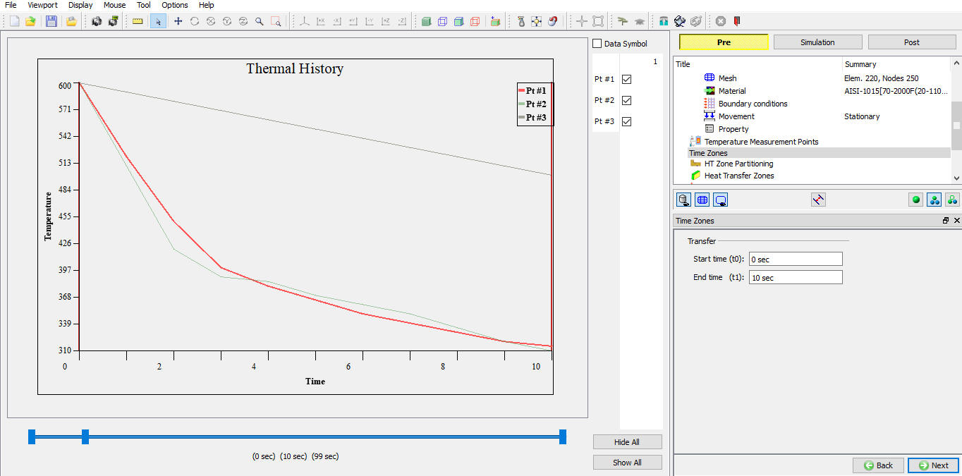
Time zone for only the Transfer process
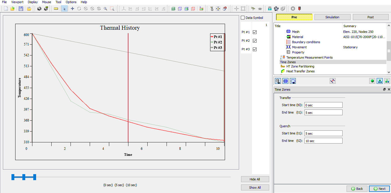
Time zone for both Transfer and Quench process
HT Zone Partitioning
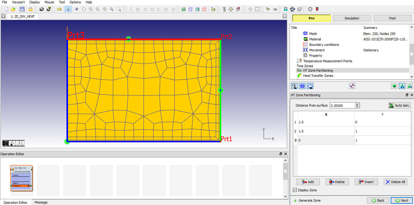
In “HT Zone Partitioning” page we can define zones over the workpiece boundary. The zones are the continuous surfaces which are exposed to similar conditions. User can define initial HTC guess and set interpolation methods for optimization of HTC values based on these zones then system calculates and optimizes the HTC values for each of these zones. System automatically generates zones based upon temperature points defined, turn on ![]() check box to verify the zones created. User can modify these zones by deleting the existing zones and adding new points over the boundary of the workpiece. To add zone, user can click on add button and select the point on the Workpiece as shown in the Fig. 51.1.18., after defining the points click on
check box to verify the zones created. User can modify these zones by deleting the existing zones and adding new points over the boundary of the workpiece. To add zone, user can click on add button and select the point on the Workpiece as shown in the Fig. 51.1.18., after defining the points click on ![]() button. Using
button. Using ![]() button we can delete all the defined zones and define new, minimum one zone must be defined else system will consider the entire surface as one zone.
button we can delete all the defined zones and define new, minimum one zone must be defined else system will consider the entire surface as one zone. ![]() button can be used to generate zones automatically.
button can be used to generate zones automatically.
Note : For Symmetry model the zones are created without considering the symmetric surfaces.
Defining the points for HT Zone Partitioning
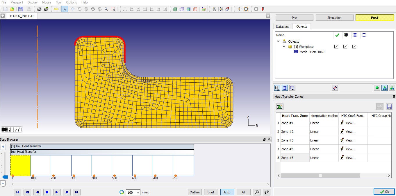
Heat Transfer Zones
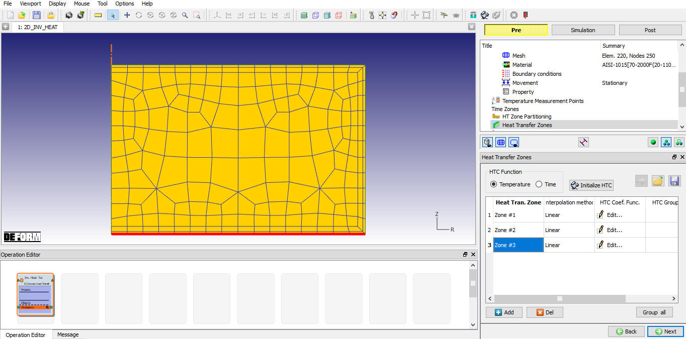
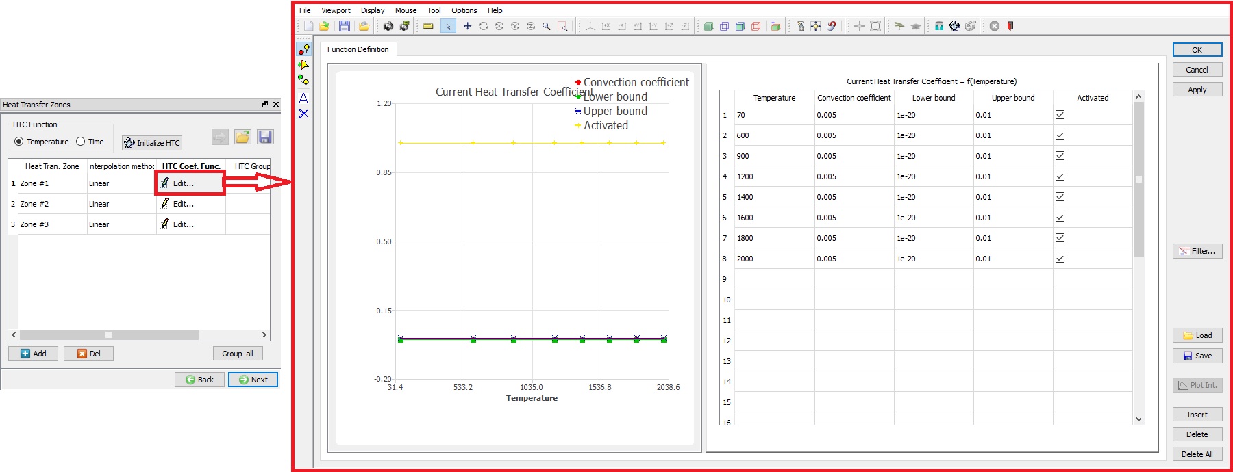
Once the zones are portioned in the HT Zone Partioning page, user can set the interpolation method and define initial HTC guess values for HTC optimization in Heat Transfer Zones page. User can set the interpolation method and define initial HTC guess values for each zone by clicking on ![]() button under “HTC Coef. Func” column as shown in Fig. 51.1.19. The function data of HTC can be function of temperature or time, user can select the appropriate function from HTC function tab as shown in Fig. 51.1.20.
button under “HTC Coef. Func” column as shown in Fig. 51.1.19. The function data of HTC can be function of temperature or time, user can select the appropriate function from HTC function tab as shown in Fig. 51.1.20.
Heat Transfer Zones page
Defined Function data page
Heat Transfer Coefficient Function Definition
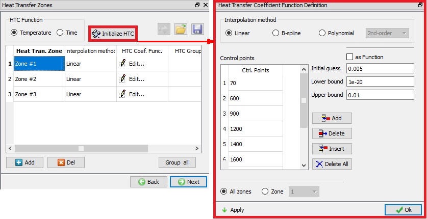
![]() button (see Fig. 51.1.21.) can be used to initialize the HTC values for all zones. Once the user clicks on “Initialize HTC” button it opens Heat Transfer Coefficient Function Definition page as shown in Fig. 51.1.21. User can define the control points used to construct temperature or time dependent HTC function. User can set the initial guess value, the minimum and maximum values for the heat transfer coefficients. Once the user initializes the data user can modify the values for each zone independently using
button (see Fig. 51.1.21.) can be used to initialize the HTC values for all zones. Once the user clicks on “Initialize HTC” button it opens Heat Transfer Coefficient Function Definition page as shown in Fig. 51.1.21. User can define the control points used to construct temperature or time dependent HTC function. User can set the initial guess value, the minimum and maximum values for the heat transfer coefficients. Once the user initializes the data user can modify the values for each zone independently using ![]() button as shown in Fig. 51.1.20. Defining a reasonable initial HTC guess values helps the DEFORM optimization routines to get to the desired results quicker. For example, defining a huge range of lower and upper bound heat transfer values for a heat treat process, and an unreasonably higher or lower initial guess, which is not representative of the quench process, would drive the optimization routine to take a longer time to solve the problem.
button as shown in Fig. 51.1.20. Defining a reasonable initial HTC guess values helps the DEFORM optimization routines to get to the desired results quicker. For example, defining a huge range of lower and upper bound heat transfer values for a heat treat process, and an unreasonably higher or lower initial guess, which is not representative of the quench process, would drive the optimization routine to take a longer time to solve the problem.
Heat Transfer Coefficient Function Definition page
Positioning
User can position the objects using ![]() button. Various positioning options are available to position the objects as shown in Fig. 51.1.22., for more information on these options please refer 2D Positioning objects.
button. Various positioning options are available to position the objects as shown in Fig. 51.1.22., for more information on these options please refer 2D Positioning objects.
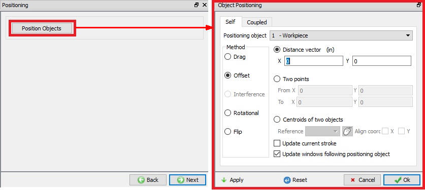
Positioning options
Step
The user can define the step definition data for the selected process. If we select any one process, then the respective process step definition will be as shown in the Fig. 51.1.23. If we select both the process, then the transfer and quench step definition will be as shown in the Fig. 51.1.24.
Number of steps (NSTEP): he number of simulation steps parameter is fixed for inverse heat wizard as 999999. The simulation will stop after the optimization is finished.
Step Increment(STPINC) : The step increment to save in the database controls the number of steps that the system will save in the database. When a simulation runs, every step must be computed, but does not necessarily need to be saved in the database. Storing more steps will preserve more information about the process, consequently it will require more storage space.
Step increment control : Time (DTMAX): If time per step is specified, the time interval per step will be used.
Temperature (DTPMAX) : If user selects the temperature-based step increment, then the time interval for step increment is controlled by the settings defined as shown in Fig. 51.1.23.
-
Temp. change per step: It specifies maximum change in the temperature allowed per step, whenever change in temperature in the object exceeds this value then time per step is reduced and whenever it is less than the specified value then the time per step is increased.
-
Min/Max Time per step: It specifies the range for time per step within which system can set the value when temperature change in the object is less than or more than “Temp. change per step” value.
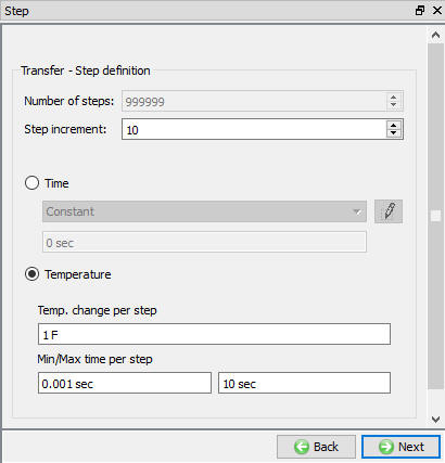
Step controls for any one Process (Transfer)
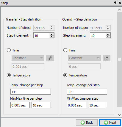
Step controls for both Transfer and Quench process
Optimization Controls
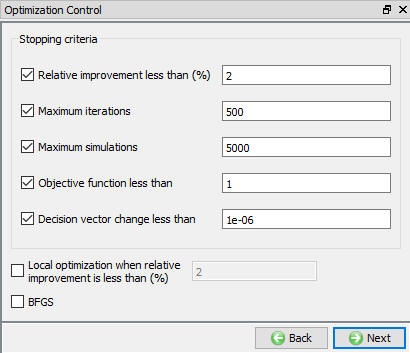
In Optimization Control user can define the criteria to stop the optimization as show in the Fig. 51.1.25.
Stopping Controls:
**Relative improvement less than (%):** When the Relative improvement in the predicted temperature curves between the current HTC values and previous HTC values is less than the defined value, then the optimization will stop.
Maximum iteration : Simulation stops when the iterations reaches the Maximum iteration value.
Maximum simulation : When the number of simulations exceeds the defined Maximum simulation value, optimization will stop.
Objective function less than : Simulation stops when the Objective function error is less than the defined “Objective function less than value”.
Decision vector changes less than : Simulation stops when the decision vector change is less than the defined “Decision vector changes less than” value.
Local optimization when relative improvement is less than (%) : By checking “Local optimization when relative improvement is less than (%)” check box, Local optimization will be carried out when the relative improvement in the temperature prediction using current HTC values compared to that of the temperature prediction using previous HTC values is less than the defined value.
BFGS : By checking BFGS (Broyden–Fletcher–Goldfarb–Shanno ) check box, optimization uses BFGS algorithm to optimize the HTC values.
Optimization Controls page
Generate DB
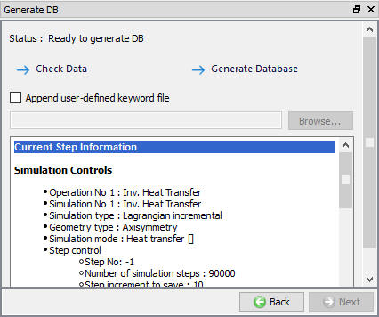
Check Data ![]() : It checks the Data. If Data is correct, we can generate DB. But while checking Data if it gives any errors or warnings then it should be corrected before generating Database. Errors will not allow the database to be generated while warnings will allow the DB to be generated.
: It checks the Data. If Data is correct, we can generate DB. But while checking Data if it gives any errors or warnings then it should be corrected before generating Database. Errors will not allow the database to be generated while warnings will allow the DB to be generated.
**Generate Database![]() : ** By clicking on this button, system generates the Database for the setup (See Fig. 51.1.26.).
: ** By clicking on this button, system generates the Database for the setup (See Fig. 51.1.26.).
Append Key file : Any information that is not defined in the wizard but still applicable to the process can be loaded as .key file. This option is also useful in the cases where only few values needs to be changed then those values can be defined as .key file and only .key file can be changed, and simulation can be resubmitted.
Generate DB page
Post-Processing the Inverse HT Optimized results
Once the optimization is completed, we can notice that there will be two DBs in the project folder, one with Project_INI.DB and other one as Project_Optimized.DB. The Project_INI.DB has initial settings defined while generating the database while Project_Optimized.DB has optimized HTCs. When user shifts to POST tab in Inverse HT wizard, we can notice two icons as shown in Fig. 51.1.27.
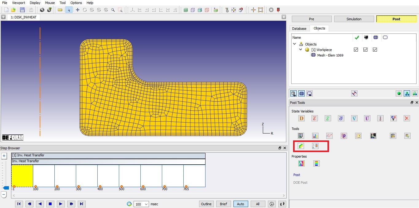
2D Inverse Heat post processor
Local Objectives![]() :
:
![]() is used to plot the experimental temperature values and predicted values in optimized solution. . When user clicks on the
is used to plot the experimental temperature values and predicted values in optimized solution. . When user clicks on the ![]() icon it opens window as shown in Fig. 51.1.27., user can click on
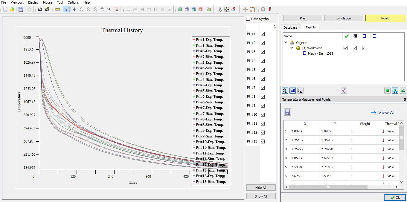
icon it opens window as shown in Fig. 51.1.27., user can click on ![]() button to display the experimental and predicted temperature curves. The plotted graphs have display controls to control the display of curves for selected points as shown in Fig. 51.1.28.
button to display the experimental and predicted temperature curves. The plotted graphs have display controls to control the display of curves for selected points as shown in Fig. 51.1.28.
Thermal history of the temperature measurement points
Optimal HTC![]() :
:
![]() is used to plot the HTC values for each zone defined in the pre-processor as function of temperature or time from the optimized solution, see Fig. 51.1.29. The HTC values can be exported from the graph and can be used in simulation of quenching or other heat treatment processes.
is used to plot the HTC values for each zone defined in the pre-processor as function of temperature or time from the optimized solution, see Fig. 51.1.29. The HTC values can be exported from the graph and can be used in simulation of quenching or other heat treatment processes.
Optimal HTC output for defined zones
For more details on other post-processing tools please refer Post processor.