Lab 4. Steering Link
4.1. Introduction
4.2. Creating New problem
4.3. Adding Operations and Objects
4.4. Defining Workpiece
4.5. Defining Top Die
4.6. Defining Bottom Die
4.7. Positioning Objects
4.8. Assigning Inter-Object Relation
4.9. Assigning Stopping Controls
4.10. Step Controls
4.11. Database Generation
4.12. Post Processing
Introduction
The German Forging Industry Association (Industrieverband Deutscher Schmieden or IDS) hosts periodic benchmark tests of forging simulation codes. These are actual industrial parts in which all process data are available for distribution.
In this lab and the next lab, the two parts from the 1999 benchmark will be used to illustrate realistic problem setup. Depending on hardware and system settings, these problems will run anywhere from several hours to a day or two. One of the keys to optimizing simulation performance is mesh definition which will be discussed in depth later in the lab.
Accurately simulating a hammer forging process requires an above normal amount of data about the press, and some additional effort to set up and run the simulation.
Creating New Problem
Create a new problem either by selecting File![]() **New Problem** or by clicking the New Problem
**New Problem** or by clicking the New Problem![]() icon. The Problem Setup window will appear. Select “Integrated Manufacturing Process “ radio button and units system as “SI “ radio button in units field. Define Problem Name as “Steering_Link “ and make sure the “Show option dialog ” check box is turned on (if we do not turn on the “Show option dialog” check box, then we will not get the New Project dialog). Then click on
icon. The Problem Setup window will appear. Select “Integrated Manufacturing Process “ radio button and units system as “SI “ radio button in units field. Define Problem Name as “Steering_Link “ and make sure the “Show option dialog ” check box is turned on (if we do not turn on the “Show option dialog” check box, then we will not get the New Project dialog). Then click on ![]() button to open a new problem using the Deform Integrated Manufacturing Process.
button to open a new problem using the Deform Integrated Manufacturing Process.
MO wizard will open, at this point user will be prompted to specify a project name (system will create a separate folder with this project name) and title for this session. In this session we use ‘Steering_Link ’ as the project name.
User can also change the Unit system and add operation by selecting from First operation pull down list and checkbox. Using copy Existing project option we can import previous saved projects as new project. Click on ![]() to continue to open the operation.
to continue to open the operation.
Adding operation and Objects
Add 3D Forming operation from the Explorer Operations list. Add the operation by clicking on 3D Forming ![]() button or user can also add by drag and drop into the Operation Editor. Click
button or user can also add by drag and drop into the Operation Editor. Click ![]() until Objects page.
until Objects page.
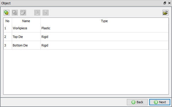
In Objects Page, by default 3 objects will be added if not add objects by selecting ![]() button, add three objects as shown in Fig. 3DL4.1. Click
button, add three objects as shown in Fig. 3DL4.1. Click ![]() .
.
Adding Objects
Defining Workpiece
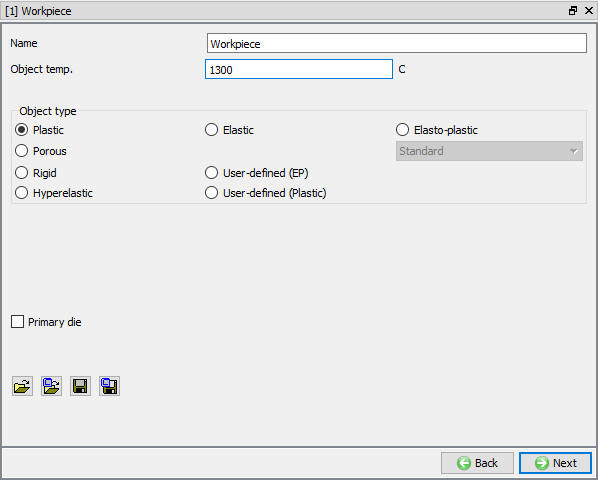
Assigning Workpiece Temperature
In Workpiece page, enter workpiece temperature as 1300 °C as shown in Fig. 3DL4.2. Click ![]() .
.
Assigning temperature for Workpiece
Import Geometry
In Geometry page, click on import geometry from library option ![]() and import the ids_link_billet.stl file from DEFORM installation folder \3d\LABS directory. Use
and import the ids_link_billet.stl file from DEFORM installation folder \3d\LABS directory. Use ![]() button to check the Geometry. A Geometry checking popup will appear in Display window as shown in Fig. 3DL4.3. Click
button to check the Geometry. A Geometry checking popup will appear in Display window as shown in Fig. 3DL4.3. Click ![]() and click
and click ![]() .
.
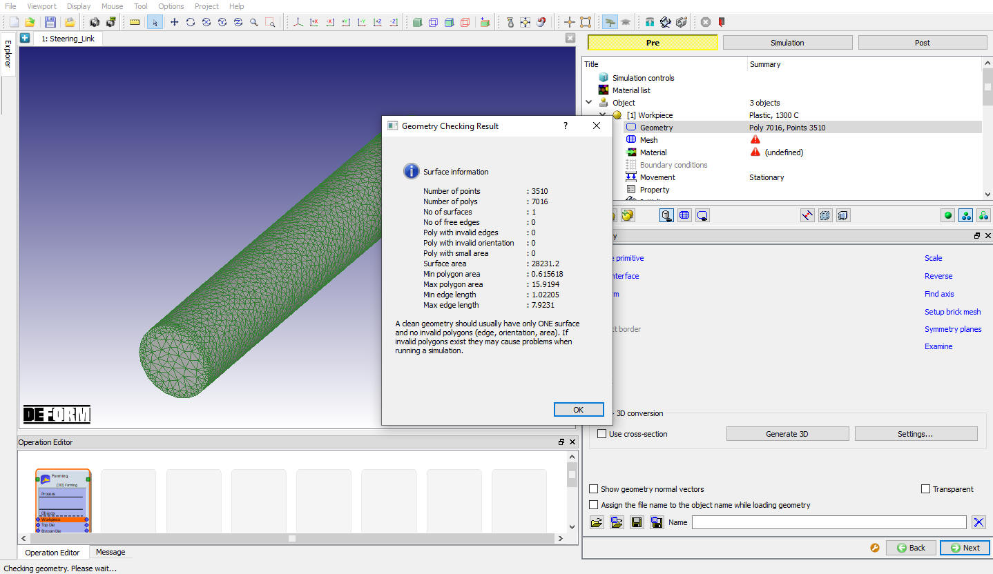
Geometry checking Window
Defining Workpiece Mesh
The workpiece mesh has the largest influence of all simulation settings on simulation accuracy and speed. A coarse mesh will allow extremely fast simulation speeds, but surface resolution will be poor. More mesh elements will enhance surface resolution, but will do so at the expense of simulation time.
In general, features and defects which are of the same order of size or smaller than the element size will not be captured.
DEFORM® offers two options for mesh description:
Absolute mesh allows the user to specify mesh resolution. The total number of mesh elements will be determined by the system, but resolution will remain constant.
Relative mesh allows the user to specify a total number of solid elements. The number of solid elements will remain relatively constant, and surface resolution will change as the simulation progresses.
In general, absolute mesh provides better performance, because for a desired resolution, the simulation uses fewer elements at the start, and adds elements as necessary to maintain resolution. Both mesh descriptions offer adaptive automatic mesh refinement – finer elements are used in areas where more resolution is required.
Mesh Density Definition for Fine Resolution
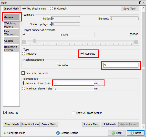
It is common to base mesh definition on feature sizes in the tooling. In the case of this part, the critical features are the blend radii leading from the shank into the eyes, and the fillets leading into the flash radius. These fillets are around 2mm. To resolve these, the minimum element size should be about ½ of this size, or 1mm.
Change the preprocessor setup mode to Expert by using the ![]() (Switch to expert mode) icon from the tool bar. In Mesh page, select absolute mesh radio button, a Minimum Element Size of 1 mm and a SizeRatio of3 should be entered as mesh parameters for the workpiece as shown in Fig. 3DL4.4.
(Switch to expert mode) icon from the tool bar. In Mesh page, select absolute mesh radio button, a Minimum Element Size of 1 mm and a SizeRatio of3 should be entered as mesh parameters for the workpiece as shown in Fig. 3DL4.4.
General Mesh Window
The weighting parameters set the relative influence of surface curvature, strain, strain rate and temperature gradient on mesh definition. Higher weights on curvature will give better boundary resolution. Change the weighting to about 0.9 for Surface Curvature and 0.1 for both Strain and Strain Rate as shown in Fig. 3DL4.5.
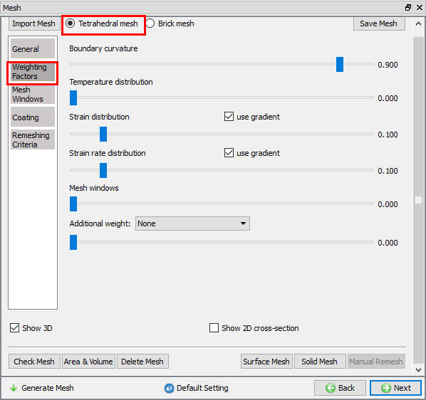
Mesh Weighing Factors window
First generate a ![]() and then a
and then a ![]() for the billet. Click
for the billet. Click ![]() for Default Boundary conditions popup. A mesh with about 76,000 solid elements will be generated. At each remesh, the defined absolute mesh settings will be maintained, so the total number of elements will increase as the geometric complexity of the workpiece increases.
for Default Boundary conditions popup. A mesh with about 76,000 solid elements will be generated. At each remesh, the defined absolute mesh settings will be maintained, so the total number of elements will increase as the geometric complexity of the workpiece increases.
Importing Material Data
In the Material window, Select steel category and load the material DIN41Cr4 using Load material data from library ![]() option as shown in Fig. 3DL4.6.
option as shown in Fig. 3DL4.6.
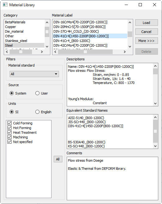
Material Window
After loading the data, click on ![]() button, Material window will open. In that window, view the thermal and plastic data by clicking on the
button, Material window will open. In that window, view the thermal and plastic data by clicking on the ![]() button next to each of the properties. Click
button next to each of the properties. Click ![]() and click
and click ![]() .
.
Assigning Boundary Conditions
Only half of the steering link is being modeled. To enforce symmetry, we need to define a symmetry plane boundary condition to the +X end of the part as shown in Fig. 3DL4.7., and heat exchange with the environment boundary condition to all surfaces except the +X end of the part as shown in Fig. 3DL4.8. and click on ![]() until Properties.
until Properties.
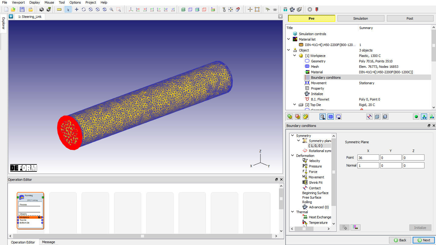
Symmetry BCC Definition
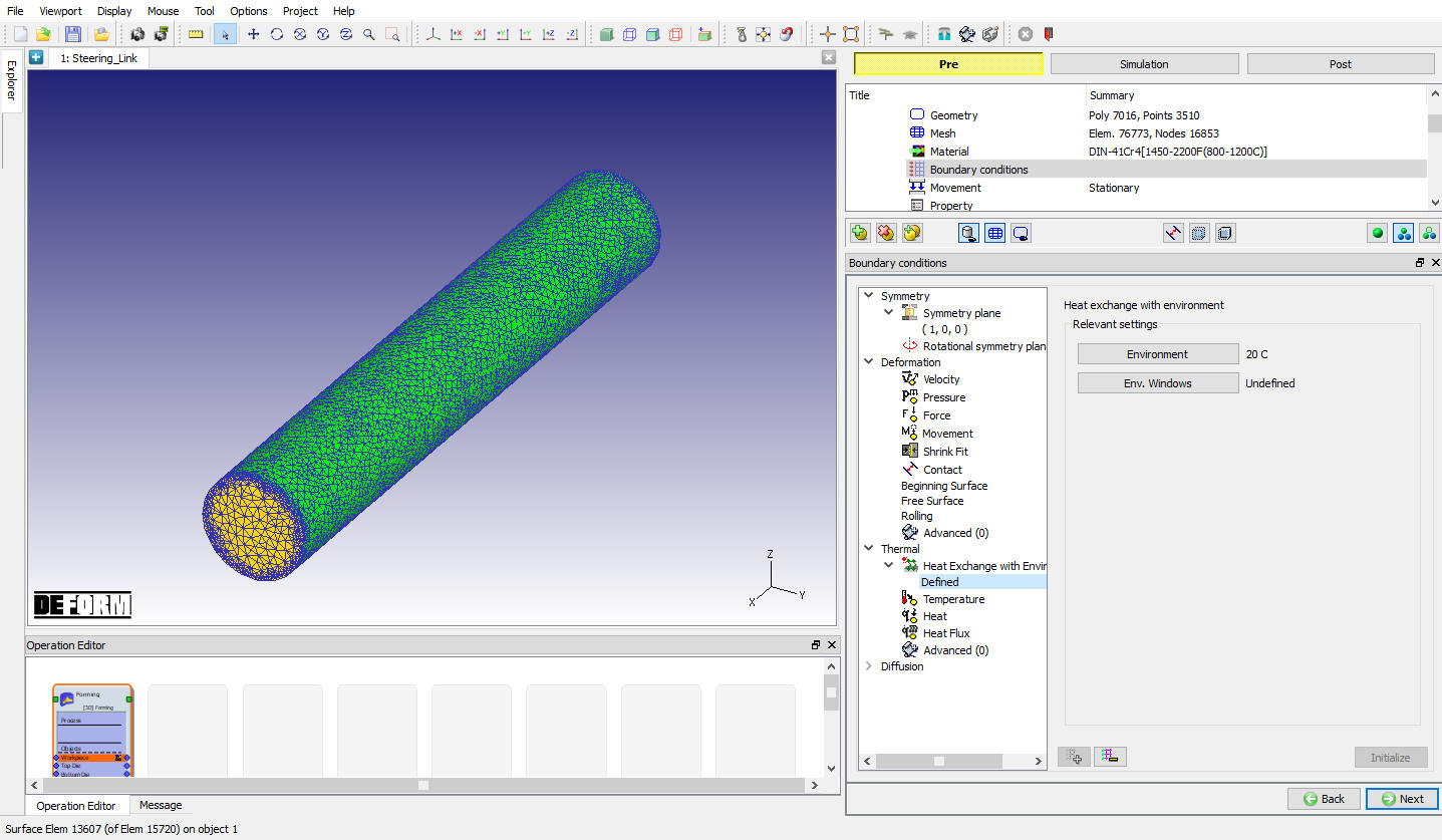
Heat Exchange with Environment BCC definition
Activating Volume Compensation
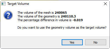
In properties page, click on the Deformation button and set the TargetVolume to Active in FEM + meshing. Click the ![]() button to calculate the volume of the workpiece mesh and geometry. In general, the mesh volume will be slightly smaller than the geometry volume. Using the geometry volume as the target volume will cause DEFORM® to gradually grow the workpiece volume back to the target. Using mesh volume at the target volume will cause DEFORM® to maintain a constant volume.
button to calculate the volume of the workpiece mesh and geometry. In general, the mesh volume will be slightly smaller than the geometry volume. Using the geometry volume as the target volume will cause DEFORM® to gradually grow the workpiece volume back to the target. Using mesh volume at the target volume will cause DEFORM® to maintain a constant volume.
When asked, use the geometry volume as the target volume by clicking ![]() button as shown in Fig. 3DL4.9.
button as shown in Fig. 3DL4.9.
Target volume popup
Click ![]() until Top Die page
until Top Die page
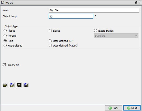
Defining Top Die
Assign Temperature
In Top Die page, assign temperature for Top Die as 90 °C s shown in Fig. 3DL4.10. then click on ![]() .
.
Assigning Top Die Temperature
Import Geometry
In Geometry page, click on import geometry from library option ![]() and import the Ids_link_top.stl file from DEFORM installation folder \3D\LABS directory. Use
and import the Ids_link_top.stl file from DEFORM installation folder \3D\LABS directory. Use ![]() button to check the Geometry. Click
button to check the Geometry. Click ![]() until movement page.
until movement page.
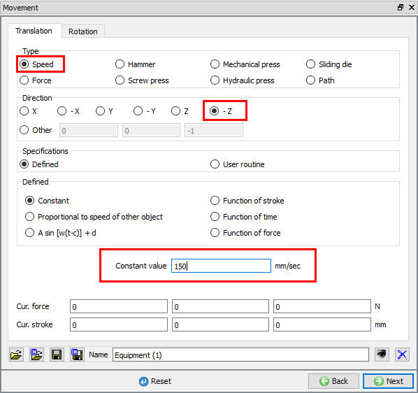
Assign Movement
For a simplified simulation, we will assign a constant top die velocity of 150 mm/s in the -Z direction (see Fig. 3DL4.11.). Click ![]() until Bottom die page.
until Bottom die page.
Movement Control Window
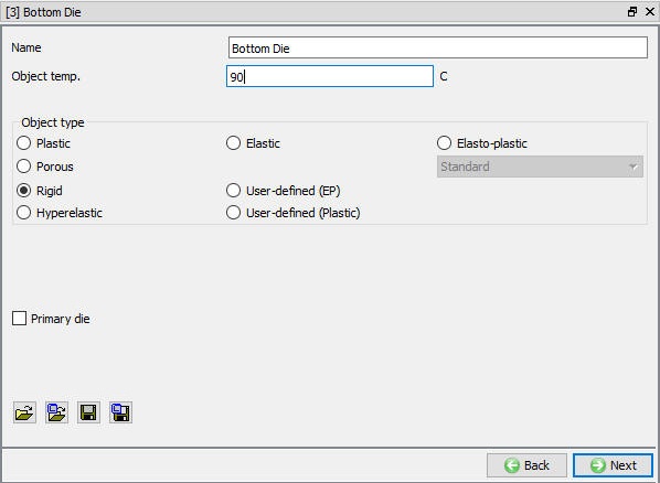
Defining Bottom Die
Assign Temperature
In Bottom Die page, assign temperature for Bottom Die as 90 °C as shown in Fig. 3DL4.12. then click on ![]() to geometry page.
to geometry page.
Assigning Bottom Die Temperature
Import Geometry
In Geometry page, click on import geometry from library option ![]() and import the ids_link_bottom.stl file from DEFORM installation folder \3D\LABS directory. Use
and import the ids_link_bottom.stl file from DEFORM installation folder \3D\LABS directory. Use ![]() button to check the Geometry. Click
button to check the Geometry. Click ![]() until Positioning page.
until Positioning page.
Positioning Objects
Click on ![]() and select
and select ![]() radio button. Change the Positioning Object to the Top Die and the Reference to the Workpiece. Change the Approach Direction to -Z and then click
radio button. Change the Positioning Object to the Top Die and the Reference to the Workpiece. Change the Approach Direction to -Z and then click ![]() .
.
Again select ![]() radio button. Change the Positioning Object to the BottomDie and the Reference to the Workpiece. Change the Approach Direction to Z and then click
radio button. Change the Positioning Object to the BottomDie and the Reference to the Workpiece. Change the Approach Direction to Z and then click ![]() . Click
. Click ![]() and click
and click ![]() until contact page.
until contact page.
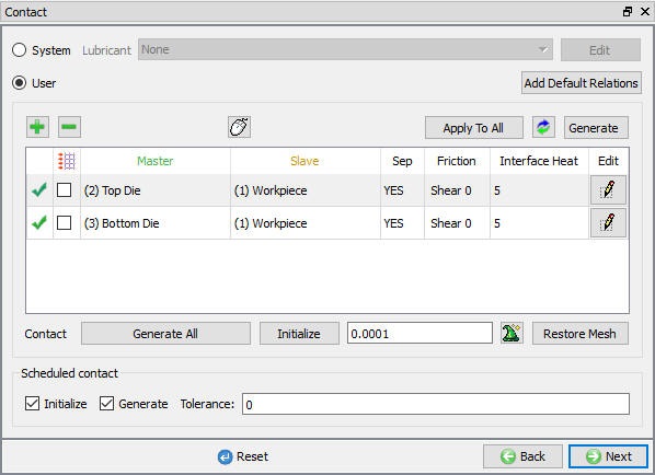
Assigning Inter-Object Relations
In Contact window, click on ![]() button, default relations get added as shown in Fig. 3DL4.13.
button, default relations get added as shown in Fig. 3DL4.13.
Inter-Object Window with Default Relations
The workpiece should be slave to both dies. Use a friction value of0.3 (typical for hot forming), and an interface heat transfer coefficient of 5 (typical for SI units when dies are not meshed).Remember to generate contact boundary conditions.
Highlight the first relationship in the table and click ![]() . On the Deformation tab, use the friction pull-down menu to select Hot forging (lubricated) from the list as shown in Fig. 3DL3.47 then click
. On the Deformation tab, use the friction pull-down menu to select Hot forging (lubricated) from the list as shown in Fig. 3DL3.47 then click ![]() .
.
Select Thermal Tab and enter an interfaceheattransfercoefficient of 5 (typical for SI units when dies are not meshed) as shown in Fig. 3DL4.14. Then click ![]() .
.
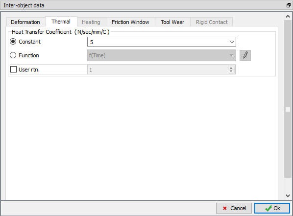
Thermal Data Definition window
In Contact window, click on ![]() to change the other relationship to these settings as shown in Fig. 3DL4.15.
to change the other relationship to these settings as shown in Fig. 3DL4.15.
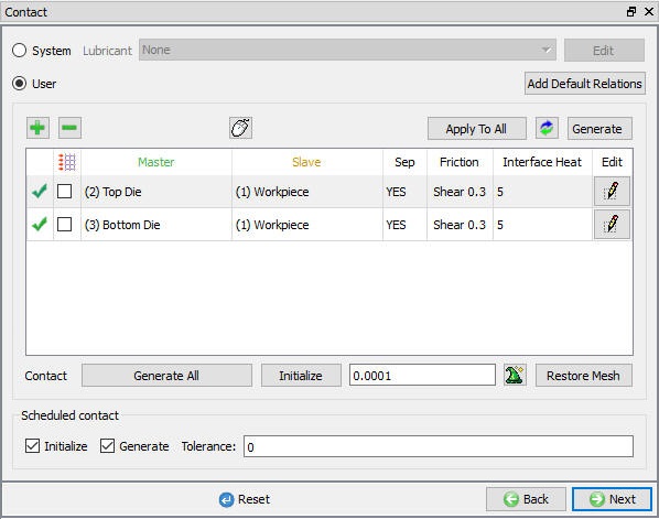
Inter-Object Window
Use ![]() to determine a suitable contact tolerance and then click the
to determine a suitable contact tolerance and then click the ![]() button to generate contacts. Contact will be generated between the Billet and both the Top and Bottom Dies. Click
button to generate contacts. Contact will be generated between the Billet and both the Top and Bottom Dies. Click ![]() .
.
Assigning Stopping Controls
Switch to Guided ![]() mode, Select
mode, Select ![]() icon, a message pop up appears in Display window, uncheck the workpiece check box in the message popup as shown in Fig. 3DL4.16.
icon, a message pop up appears in Display window, uncheck the workpiece check box in the message popup as shown in Fig. 3DL4.16.
User Define Object mode
In Stopping Controls window, Check the Distance between Objects check box. For Object 1, select Top Die and click the button ![]() . Select a point on the bottom of the Top Die. For Object 2, select Bottom Die and click the
. Select a point on the bottom of the Top Die. For Object 2, select Bottom Die and click the ![]() button. Select a point on the top of the Bottom Die. It calculates the distance and displays it in Display window. Specify a ZDistance of 11.0 mm as the stopping criteria as shown in Fig. 3DL4.17. Click
button. Select a point on the top of the Bottom Die. It calculates the distance and displays it in Display window. Specify a ZDistance of 11.0 mm as the stopping criteria as shown in Fig. 3DL4.17. Click![]() .
.
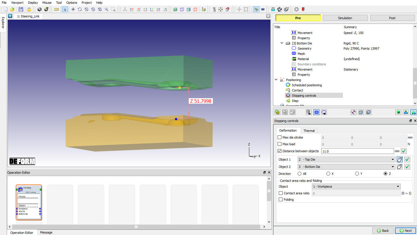
Stopping Controls window
Step Controls
The total stroke will be approximately 40mm. For a complex flash operation, 200 time steps is reasonable. The selection of this number is not critical, because sub-stepping settings will control the actual step size used in deformation calculations. In Step controls window change the preprocessor setup mode to Expert by using the ![]() (Switch to expert mode) icon from the tool bar.
(Switch to expert mode) icon from the tool bar.
In Step controls, select ![]() and assign Number of Simulation steps as 200 and stepincrementtosave10 steps. Set the TopDie as the primarydie. (See Fig. 3DL4.18.)
and assign Number of Simulation steps as 200 and stepincrementtosave10 steps. Set the TopDie as the primarydie. (See Fig. 3DL4.18.)
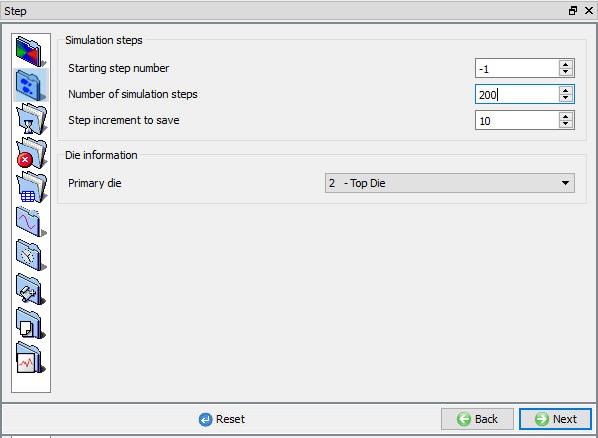
Steps Window
Select ![]() assign a stroke/step value of 0.2 mm/step as shown in Fig. 3DL4.19.
assign a stroke/step value of 0.2 mm/step as shown in Fig. 3DL4.19.
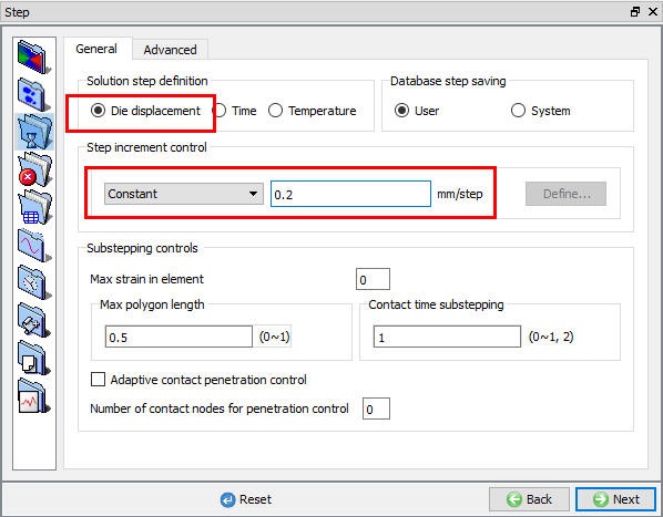
Step Controls window
Database Generation
Save a keyword file for the problem by selecting the File menu ![]() Export option.
Export option.
Click on ![]() action label to check the problem. Generate a database by clicking
action label to check the problem. Generate a database by clicking ![]() action label.
action label.
Once the database has been generated switch to the Simulation mode by selecting the ![]() button above the object tree. Click on the
button above the object tree. Click on the ![]() action label to open the Run Options dialog Use the default Continue Run option to select “Continue from the last step ” option and then select the Simulation mode as Interactive and click on
action label to open the Run Options dialog Use the default Continue Run option to select “Continue from the last step ” option and then select the Simulation mode as Interactive and click on ![]() button to run the simulation.
button to run the simulation.
Post processing
When the simulation is complete, review the results by switching to Post mode using the ![]() button above the Simulation tool bar.
button above the Simulation tool bar.
Play through the Steps and plot the Temperature, Stress Effective, Damage and Effective Strain State variables. (See Fig. 3DL4.20. and Fig. 3DL4.21.)
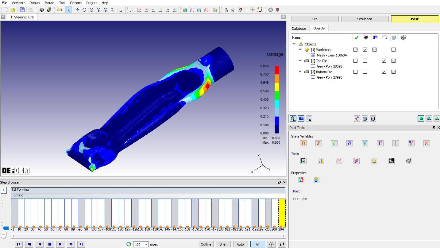
Damage State Variable plot
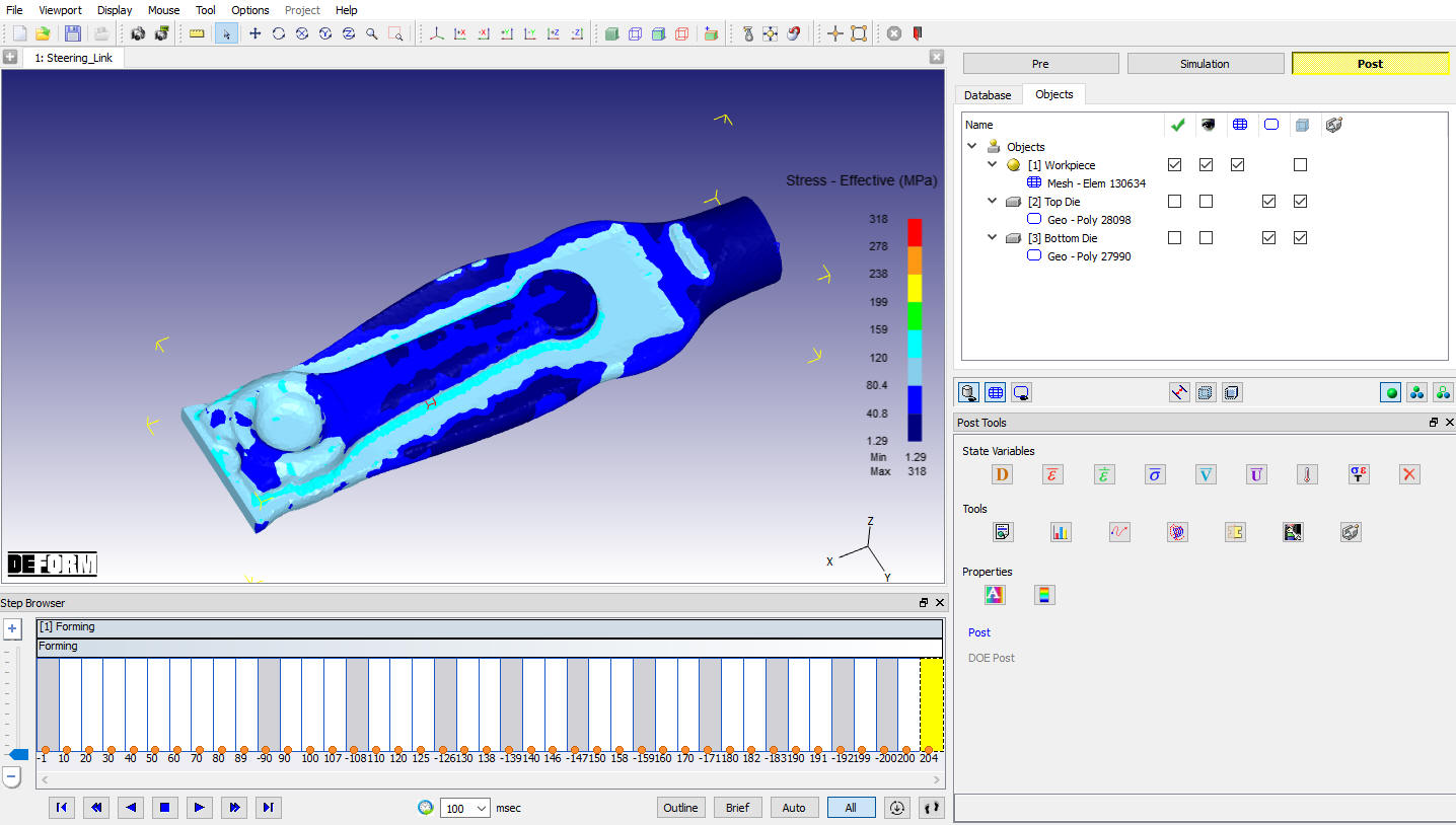
Stress Effective State Variable Plot
Click on the ![]() icon. When the GRAPH window appears, select only Top Die and the X-Axis is set to Stroke and the Y-Axis is set to Z Load. Click
icon. When the GRAPH window appears, select only Top Die and the X-Axis is set to Stroke and the Y-Axis is set to Z Load. Click ![]() and a transparent Load-Stroke curve will display over the objects in the DISPLAY window as shown in Fig. 3DL4.22.
and a transparent Load-Stroke curve will display over the objects in the DISPLAY window as shown in Fig. 3DL4.22.
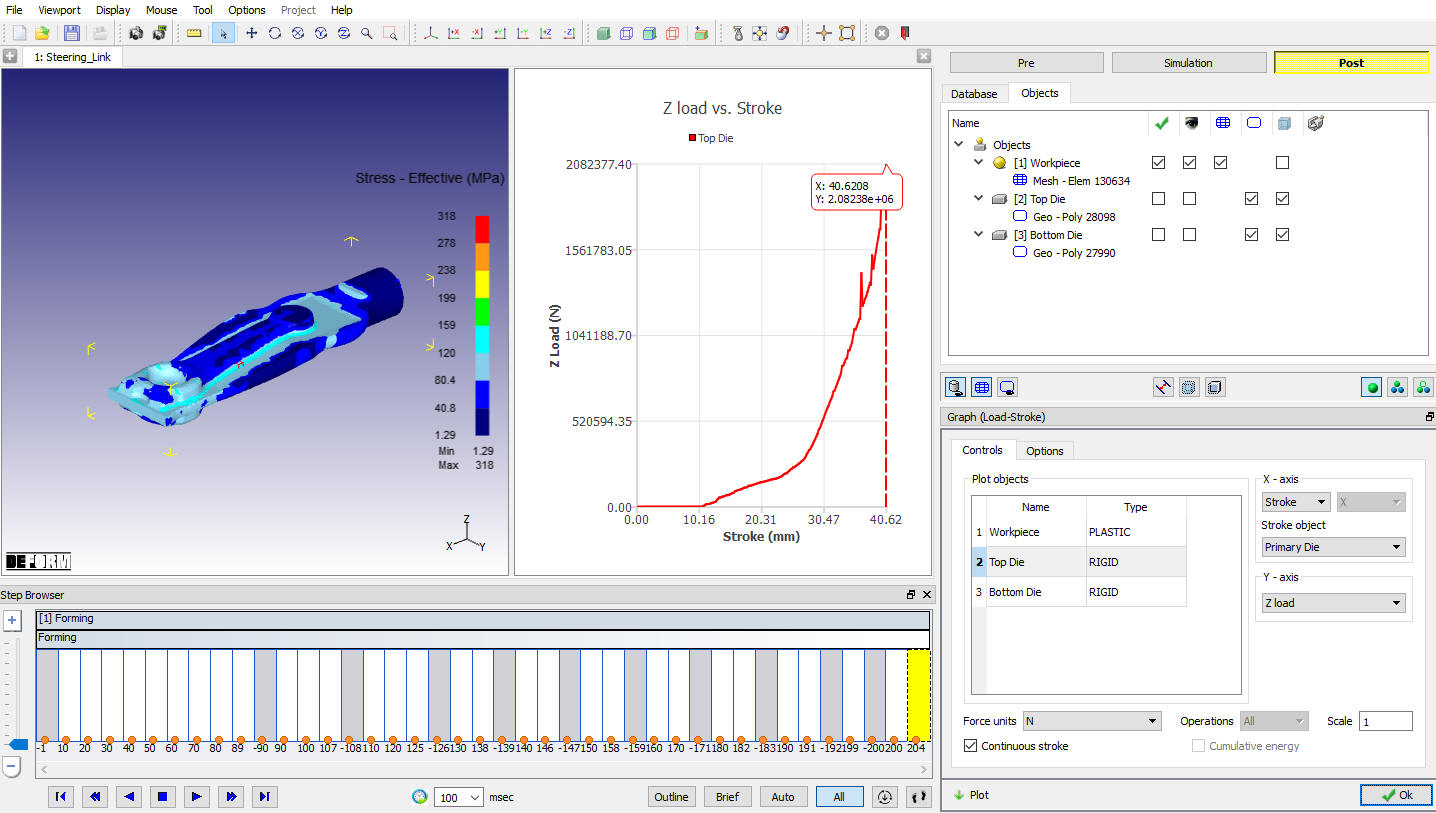
Load Stroke graph
Viewing die fill:
There are several methods of evaluating die fill in the Post-processor.
The nodes which are in contact with dies can be shown by highlighting the workpiece in the Object Tree and clicking ![]() to view contact. Areas of unfill can be recognized by lack of contact. View the part at various steps to watch the contact evolve.
to view contact. Areas of unfill can be recognized by lack of contact. View the part at various steps to watch the contact evolve.
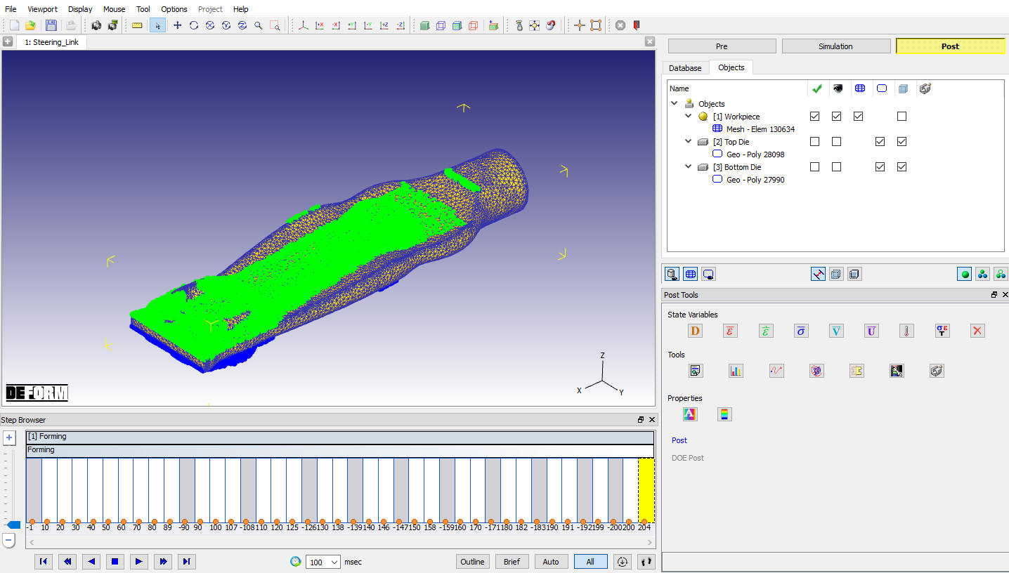
Area viewing Die fill