Lab for MEDC model (microstructure evolution during cooling) for titanium alloys
1.1. Overview
1.2. Launch MEDC model in material suite
1.3 Object selection and point selection
1.4 Setup for MEDC model
1.5 Run material point simulator
1.6 Output
Overview
The MEDC (Microstructure Evolution During Cooling) model in material suite is applicable to titanium alloys. The objective is to model the microstructure evolution during cooling for a dual-phase alpha and beta Ti 6-4 alloy to predict transformation texture. MEDC model predicts primary alpha grain size, volume fractions of primary alpha, beta, and secondary alpha, and texture of secondary alpha transformed from beta according to the variant selection rule. Two variant selection rules are implemented in DEFORM, namely, random variant selection and preferred variant selection rule to best match the pole figures of primary alpha. The texture can be represented either in Rodrigues space or Euler space. The input data to MEDC model include MEDC simulation control data, material definition, phase transformation data from beta to primary alpha and from beta to secondary alpha, initial texture, initial volume fractions of alpha and beta phase, and initial primary alpha grain size. For each saved step in the DEFORM database, the output data include the aforementioned microstructure features. Texture analysis tools are provided, such as pole figures, inverse pole figures, and Kearns number of HCP crystal, particularly for total alpha.
The MEDC model can be run either after completing deformation texture model or as a standalone transformation texture model using known or assumed deformation texture. MEDC model can be run after finishing the deformation texture model in Material Suite so that the predicted deformation texture can be used as input into MEDC model as the initial texture. If MEDC is used as a standalone model to predict transformation texture without having any prior deformation texture model results, then user can use a typical heat treatment DEFORM database along with either measured deformation texture (EBSD) or assumed deformation texture data as the starting initial texture for the MEDC model.
In this lab, the microstructure and texture evolution during heat treatment of Ti 6-4 double cone sample setup as a standalone MEDC model is presented. This lab uses a DEFORM key file to run a heat treatment simulation and demonstrates how to use MEDC model to run a point mode simulation for transformation texture using the DEFORM database for the double cone Ti 6-4 heat treatment case using assumed deformation texture as initial starting texture.
Launch MEDC model in material suite
On a Windows machine, go to the ![]() button, select DEFORM-v12.xxx (.xxx indicates version number E.g. v14.0.2 and select DEFORM GUI Main v1x.xx from the menu. The DEFORM GUI Main window will appear.
button, select DEFORM-v12.xxx (.xxx indicates version number E.g. v14.0.2 and select DEFORM GUI Main v1x.xx from the menu. The DEFORM GUI Main window will appear.
We require a nominal DB to perform texture analysis in material suite, for this lab we will use **Double_Cone_Cooling_Nominal.key** from **\MANUALS\PDF\DEFORM3D_MEDC_Lab** folder to generate nominal DB. Open NG Pre using the link DEFORM GUI Main and define Problem ID as “ **Double_cone_Cooling ** “, select “3D “ Dimension radio button and “System International (SI) “ unit System radio button in New Problem window, then import **Double_Cone_Cooling_Nominal.key** from **\MANUALS\PDF\DEFORM\ 3D_MEDC_Lab** folder. Navigate to Generate DB page and click on ![]() to generate database. Close the NG Pre and run the simulation from GUI Main, make sure simulation stops normally without any issue. Now from GUI Main, without selecting **Double_cone_Cooling ** ** .DB file click on **MaterialSuite under “Post Processor” to open Material Suite module.
to generate database. Close the NG Pre and run the simulation from GUI Main, make sure simulation stops normally without any issue. Now from GUI Main, without selecting **Double_cone_Cooling ** ** .DB file click on **MaterialSuite under “Post Processor” to open Material Suite module.
After the main window for material suite pops up, click “Open…” icon (![]() ) in the top tool bar to import the example database (Double_cone_Cooling.DB). The default task item “DEFORM” is added to the task tree. Expand “Microstructure “ item and click “MEDC Model “ icon, the new task item “Microstructure evolution during cooling model of Ti alloy “ is added to the task tree as shown in Fig. MEDCL.1, .
) in the top tool bar to import the example database (Double_cone_Cooling.DB). The default task item “DEFORM” is added to the task tree. Expand “Microstructure “ item and click “MEDC Model “ icon, the new task item “Microstructure evolution during cooling model of Ti alloy “ is added to the task tree as shown in Fig. MEDCL.1, .
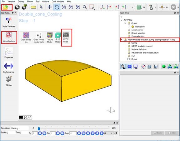
Launch MEDC model in material suite.
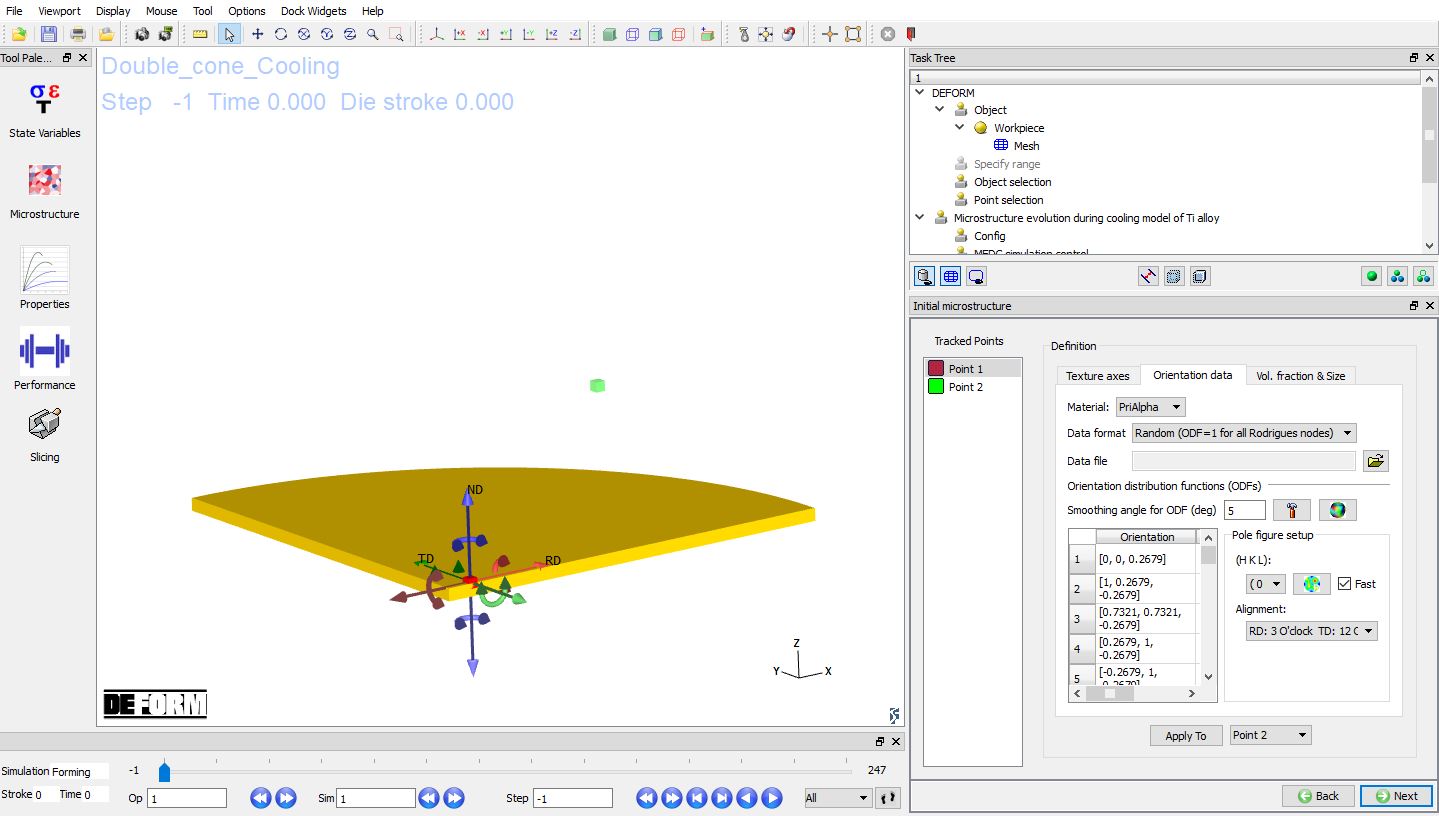
Object selection and point selection
As shown in Fig. MEDCL.2, in the “DEFORM” task tree, click “Object selection “ item and select “Workpiece “. Click “Point selection “, define step number as “-1” and define two points on the workpiece (Fig. MEDCL.3). The coordinate of point 1 (P1) is (1.176, 0, 0.381, 1), and the coordinate of Point 2 (P2) is (8.950, 0, 8.701, 1).
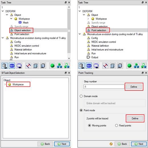
Object selection and point selection
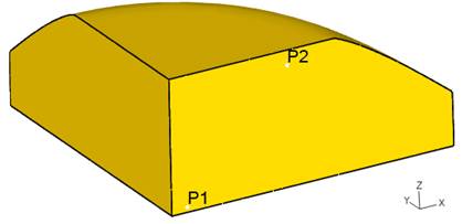
Points definition on workpiece
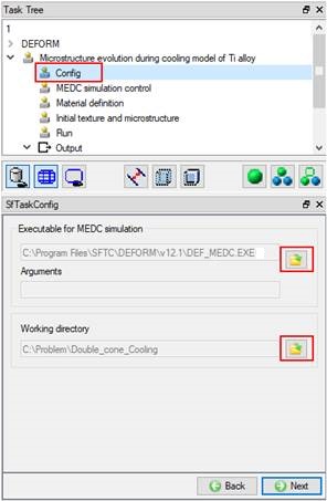
Configuration
Setup for MEDC model
All data for MEDC model are prepared by the items in the “Microstructure evolution during cooling model of Ti alloy “ task tree. Refer to Fig. MEDCL.4, click “Config “ item, its data window appears. Specify the executable for MEDC simulation and the working directory by clicking the definition buttons (![]() ). The default executable for MEDC simulation is DEF_MEDC.EXE”, which is located at the installation directory of DEFORM software. Users can also develop their own executable for MEDC simulation and specify the file name here. The working directory must be the one where the nominal database is located.
). The default executable for MEDC simulation is DEF_MEDC.EXE”, which is located at the installation directory of DEFORM software. Users can also develop their own executable for MEDC simulation and specify the file name here. The working directory must be the one where the nominal database is located.
MEDC simulation control
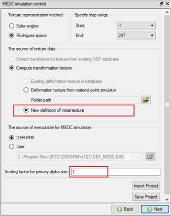
Click “MEDC simulation control “ item, its data window is shown as Fig. MEDCL.5. The following data need to be specified: texture representation method (Euler angles or Rodrigues space), the step range to apply MEDC simulation, the source of texture data, the source of executable, scaling factor for primary alpha size. The default values are provided, but users can change these values. If the texture data (ODF) exist in the database, it will be detected automatically and the user can select the radio button “Extract transformation texture from existing ODF database “. In this case, we just extract the data and display in the subsequent pages. However, if users want to recalculate the transformation texture, select the radio button “Compute transformation texture “ and select the radio button “Existing deformation texture in database “.
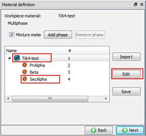
When the radio button “Compute transformation texture “ is checked, there are three choices for defining the source of deformation texture as initial texture data for MEDC model: (1) Existing deformation texture in the DEFORM database; (2) Deformation texture as a result of running DEFORM Material Suite point simulator; (3) New definition of initial texture for MEDC model. For using deformation texture from DEFORM Material suite point simulator, we need to specify the folder path of deformation texture simulation result. If this folder named “TEXTURE” exists in the current working directory, it is automatically detected and displayed in the line editor. The scaling factor of primary alpha converts the display result of primary alpha size. In this Lab, we select initial texture source 3 (New definition of deformation texture). Import material data from **Double_Cone_Cooling_Nominal.key** file using ![]() option. Check Mixture material check box and click trice
option. Check Mixture material check box and click trice ![]() button to three Phases in the list, then rename the phases as “PriAlpha “, “Beta “ and “SecAlpha “ respectively as show in Fig. MEDCL.6.
button to three Phases in the list, then rename the phases as “PriAlpha “, “Beta “ and “SecAlpha “ respectively as show in Fig. MEDCL.6.
Material definition
Click “Material definition “ item and the data window is shown in Fig. MEDCL.6. If the radio button “Extract transformation texture from existing ODF database” in MEDC simulation control page is selected, which means the texture data of secondary alpha exist in database, the material data are extracted automatically from database and displayed. The material properties can be viewed by clicking ![]() button (see Fig. MEDCL.6). In this case, the material properties should not be changed. The only concerned properties are the basic texture information (crystal type, texture type, and Rodrigues mesh type) for phase material and phase transformation data defined in parent material.
button (see Fig. MEDCL.6). In this case, the material properties should not be changed. The only concerned properties are the basic texture information (crystal type, texture type, and Rodrigues mesh type) for phase material and phase transformation data defined in parent material.
If the radio button “Compute transformation texture” in MEDC simulation control page is selected, the material definition is illustrated in Fig. MEDCL.7~10, depending on the option of initial texture source data. If the radio button “existing deformation texture in database” is selected, the texture data of primary alpha and beta are extracted from database. If texture data of secondary alpha and phase transformation data have been defined in database, these data are extracted automatically; otherwise, these data need to be defined.
If the radio button “Deformation texture from material point simulator” is selected, the texture data of primary alpha and beta are extracted automatically from the last step of material point simulator results for the deformation texture run; the texture data of secondary alpha and phase transformation data need to be defined.
If the radio button “New definition of initial texture “ is selected, the basic texture information of all phases and phase transformation data need to be defined. Fig. MEDCL.7 shows the definition of basic texture information of primary alpha and beta. The basic texture information of secondary alpha (SecAlpha) is defined in the same way as primary alpha (PriAlpha). For primary alpha and secondary alpha, the crystal type is HCP; for beta, the crystal type is BCC. For each phase, the texture representation type is Rodrigues space, and texture mesh type is type 3.
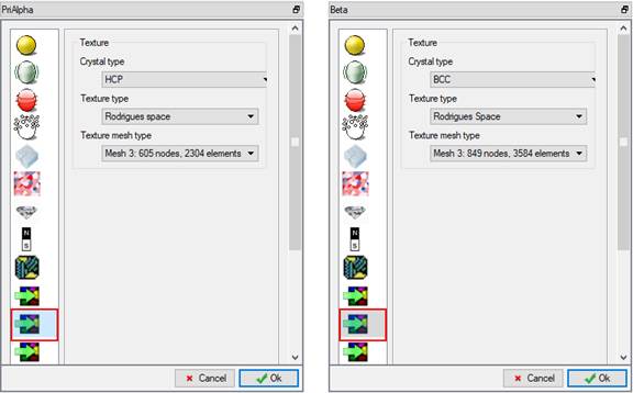
Basic texture information of each phase
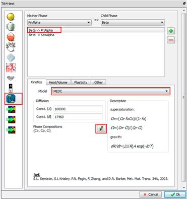
In order to define the phase transformation data, select the parent material “Ti64-test “ and click ![]() button (see Fig. MEDCL.6). In the properties window, click the transformation item icon (
button (see Fig. MEDCL.6). In the properties window, click the transformation item icon (![]() ), as shown in Fig. MEDCL.8. Add two phase transformation models: beta to primary alpha and beta to secondary alpha. For the transformation from beta to primary alpha, select “MEDC” as the kinetics model. MEDC model predicts the evolution of primary alpha size and volume fraction during cooling. The kinetics is controlled by the diffusion of vanadium or aluminum.
), as shown in Fig. MEDCL.8. Add two phase transformation models: beta to primary alpha and beta to secondary alpha. For the transformation from beta to primary alpha, select “MEDC” as the kinetics model. MEDC model predicts the evolution of primary alpha size and volume fraction during cooling. The kinetics is controlled by the diffusion of vanadium or aluminum.
The diffusion coefficient used here are adopted from (S.L. Semiatin, S.L. Knisley, P.N. Fagin, F. Zhang, and D.R. Barker, “Microstructure evolution during alpha-beta heat treatment of Ti-6Al-4V”, Metall. Mater. Trans. A34 (2003), 2377-2386).
Assuming the diffusion is controlled by vanadium, A =100000  m2/s, and B=17460 for SI unit. Click the button (
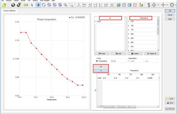
![]() ) to define the phase compositions of the diffusion-controlling element at the equilibrium state, as shown in Fig. MEDCL.8. The input quantities include; (1) the average concentration of diffusion-controlling element (V) C0: 0.042; (2) the temperatures values; (3) chemical compositions in the equilibrium state at different temperatures, which are defined by clicking “Cp” and “Ci” buttons. “Cp” represents the concentration of diffusion-controlling element in the primary alpha, and “Ci” denotes the corresponding concentration in beta phase.
) to define the phase compositions of the diffusion-controlling element at the equilibrium state, as shown in Fig. MEDCL.8. The input quantities include; (1) the average concentration of diffusion-controlling element (V) C0: 0.042; (2) the temperatures values; (3) chemical compositions in the equilibrium state at different temperatures, which are defined by clicking “Cp” and “Ci” buttons. “Cp” represents the concentration of diffusion-controlling element in the primary alpha, and “Ci” denotes the corresponding concentration in beta phase.
The detailed values for Cp and Ci as functions of temperature are provided in S.L. Semiatin, S.L. Knisley, P.N. Fagin, F. Zhang, and D.R. Barker, “Microstructure evolution during alpha-beta heat treatment of Ti-6Al-4V”, Metall. Mater. Trans. A34 (2003), 2377-2386.
In this Lab, we can also click ![]() button to load data file “Ti64_ChemicalComp.dat ” to fill in this function data. (See Fig. MEDCL.9)
button to load data file “Ti64_ChemicalComp.dat ” to fill in this function data. (See Fig. MEDCL.9)
Phase transformation data from beta to primary alpha - MEDC model selection
loaded MEDC function data from Ti64_ChemicalComp.dat file
For the phase transformation from beta to secondary alpha, select “Secondary alpha lath-based on the critical cooling rate” as the kinetics model (Fig. MEDCL.10). This model calculates the critical cooling rate for the formation of secondary alpha, and the evolution of volume fractions of beta and secondary alpha. The line to define the stating temperature ( ) and time (t) for the secondary alpha growth from the solution temperature is defined as,
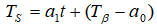
Where  is beta transus. The volume fraction of secondary alpha is calculated as
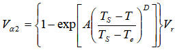
Where  is the ending temperature for the transformation from beta to secondary alpha, and
  is the balanced volume fraction of primary alpha.
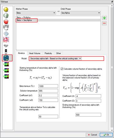
Phase transformation data from beta to secondary alpha.
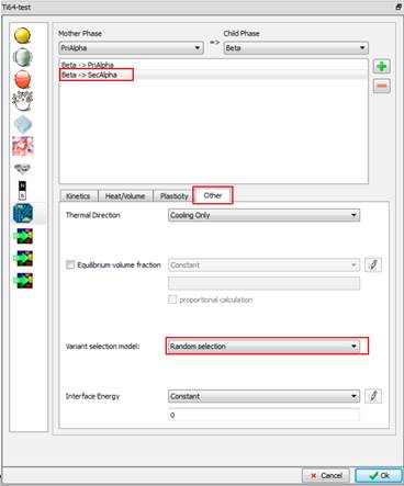
Variant selection model for phase transformation texture.
In order to define the phase transformation texture model from beta to secondary alpha, click the “other” tab shown in Fig. MEDCL.11, and select “Random selection” as the variation selection model. According to this rule, all variants are assumed to be equally likely.
We assume the following values for the demonstration purpose for this lab.
=1000°C, Solution temperature = 955 °C
 =0.2,
=0.2,  =150 °C
Temperature range above and below to calculate cooling rate:  = 50 °C
A=-4, D=3, = 500 °C
It should be mentioned that the above values of , , , A, D, and are made up values for the sake of demonstration. Users need to tune their experimental data to find the appropriate values for these parameters.
Initial texture and microstructure (overall view)
Initial texture and microstructure: texture axes
Initial texture and microstructure: ODF of primary alpha
Initial texture and microstructure: ODF of beta
Initial texture and microstructure: volume fractions and grain size
Click “Initial texture and microstructure “ item to open its data window (Fig. MEDCL.12). If the radio button “Extract transformation texture from existing ODF database” in MEDC simulation control page is selected, all data are automatically extracted and filled in this page. The data can be reviewed but cannot be modified. When the radio button “Compute transformation texture” is selected, if the initial texture is from existing ODF in database or from the deformation texture of the material point simulator, the texture data of primary alpha and beta are extracted automatically and displayed. When the radio button “new definition of initial texture” is selected, we need to define texture axes, initial texture, initial volume fraction and grain size (refer to Fig. MEDCL.12~16).
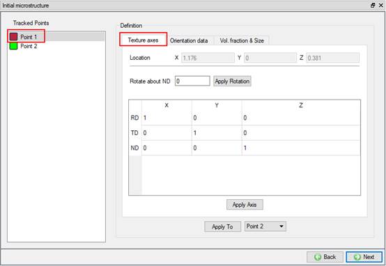
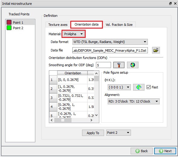
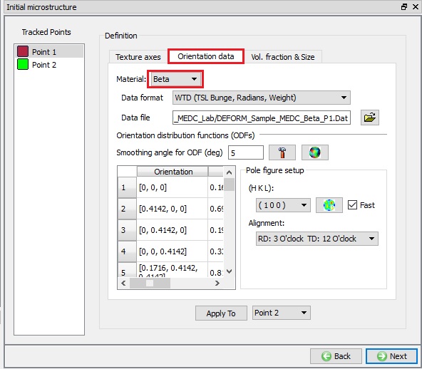
For this lab, we are going to assume and define deformation texture as starting texture for MEDC model. Refer to Fig. MEDCL.13, for Point 1, click “Textureaxes ” tab to specify the texture axes as the global coordinate axes, i.e., RD=(1,0,0), TD=(0,1,0), and ND=(0,0,1). Click “Orientationdata ” tab to initialize ODF values for each phase (Fig. MEDCL.14~15). Set data format type to 5 (WTD: TSL Bunge, Radians, Weights), and set the smoothing angle of ODF to 5 degrees. For Point 1, the initial texture data for primary alpha and beta are located in the MEDC lab folder: DEFORM_Sample_MEDC_PrimaryAlpha_P1.Dat ,
DEFORM_Sample_MEDC_Beta_P1.Dat. Click ![]() button to import data file and click on
button to import data file and click on ![]() button to calculate ODF values. For secondary alpha, use data format type 1 (random texture) to initialize ODF values so that ODF=1 for each component.
button to calculate ODF values. For secondary alpha, use data format type 1 (random texture) to initialize ODF values so that ODF=1 for each component.
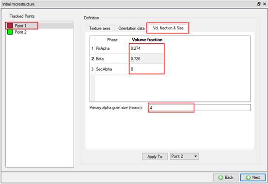
Fig. MEDCL.16 shows the definition of initial volume fraction of each phase and the initial primary alpha size (radius). In this lab, the initial volume fractions of primary alpha, beta and secondary alpha at solution temperature are 0.274, 0.726, and 0, respectively; the primary alpha size (radius) is 4 microns.
For Point 2, follow the same procedure to specify the initial texture and microstructure. Except the initial texture, the other items are the same as that of Point 1. The initial texture data for primary alpha and beta for Point 2 are located in the MEDC lab folder: DEFORM_Sample_MEDC_PrimaryAlpha_P2.Dat , DEFORM_Sample_MEDC_Beta_P2.Dat.
Run material point simulator
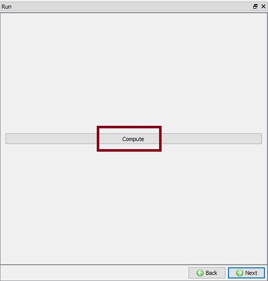
Click “Run “ item in the task tree and click “Compute “ button in the data window (Fig. MEDCL. 17). In the working directory, a folder named “MEDC_Model” will be created, and under it, the folder for each selected point named “Point” ( denotes for point number) will be created to save the simulation results.
Run simulation
Generally, the following data files are created for each selected point
(1) Input files for MEDC simulation executable:
STEP.txt : the saved step numbers in nominal database.
temp_mean.txt: The unit system and the history of temperature.
StressStrain.txt : The history of stress and strain components.
SIMCTRL_MEDC.DAT : MEDC simulation control data
MAT_MEDC.DAT : material parameters for MEDC model
TxrInfo.txt : The basic texture information and initial volume fractions for all phases
RDTDND.txt : The initial texture axes.
ODF_S-1.txt : The initial ODF values
EulerAng_S-1.txt : The initial Euler angles and weights
InitGSize.txt : The initial grain size of primary alpha
(2) Output files from MEDC simulation executable:
ODF_FS.txt : The final ODF values for primary alpha, beta, and secondary alpha
EulerAng_FS.txt : The final Euler angles and weights for primary alpha, beta, and secondary alpha
HTRES.txt : the microstructure data for all saved steps in nominal database (Step number, primary alpha particle size, volume fractions of primary alpha, beta, secondary alpha, and total alpha, the starting temperature for the formation of secondary alpha, and the critical cooling rate for the formation of secondary alpha).
(3) For multi-phase titanium alloys, the following data are outputted:
PrimAlphaSize.Dat : the initial and final primary alpha size
FinalTexture.Dat : The final texture data for primary alpha, beta, and total alpha in Bunge’s notation in radians.
Output
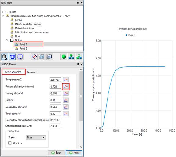
After simulation is finished, all of the selected points are listed under the “Output “ item in the task tree. Specify a step number in the step browser (should be within the range defined in the MEDC simulation control page) and select a point, the simulation results can be reviewed. Fig. MEDCL.18 shows the values of state variables at the last step and we can plot the curve of each state variable versus time or temperature. These state variables include (1) temperature, (2) primary alpha size, (3) primary alpha volume fraction, (4) beta volume fraction, (5) secondary alpha volume fraction, (6) total alpha volume fraction, (7) Secondary alpha starting temperature, (8) the critical cooling rate for the formation of secondary alpha.
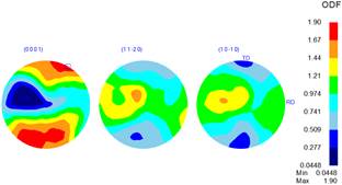
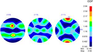
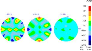
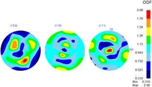
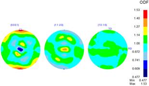
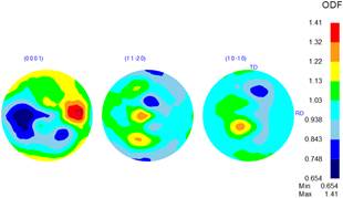
Fig. MEDCL.19 shows the GUI to display texture data and texture analysis tools. In order to carry out texture analysis, the texture axes need to be specified in the global coordinate system. Their values might be different from the initial texture axes defined in the “Initial texture and microstructure” page. Here the RD is aligned in global X direction, TD global Z direction, and ND global negative Y direction. Fig. MEDCL.19 is also an example for setup to analyze the texture of total alpha. Fig. MEDCL.20 plots the pole figures of primary alpha, beta, secondary alpha, and total alpha at Point 1; Fig. MEDCL.21 plots pole figures at Point 2. By comparing the pole figures of secondary alpha and beta, strong Burgers relation between beta and secondary alpha is observed, i.e., (0001) // (110)
 , and <11-20> // <111>.
Output: State variable and its evolution
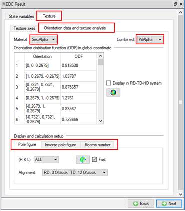
Output: orientation data and texture analysis tools to plot ODF contour, pole figures, inverse pole figures, and calculation of Kearns number for HCP phase. This GUI is also an example to plot the pole figures of total alpha.
(a)
(b)
(c)
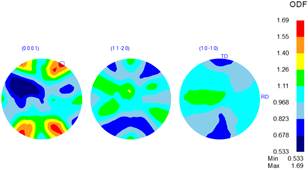
(d)
Output: pole figures for Point 1: (a) primary alpha; (b) beta; (c) secondary alpha; (d) total alpha
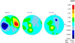
(a)
(b)
(c)
(d)
Output: pole figures for Point 2: (a) primary alpha; (b) beta; (c) secondary alpha; (d) total alpha