ALE Extrusion Lab1
In this Lab we are setting up a operation of ALE extrusion. We will also introduce the acceleration updating of state variables, and compare its simulation result with that of without acceleration updating in this Lab.
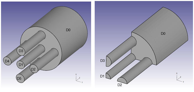
The application of this lab will extrude 5 small cylinder parts from a large cylinder billet. The model of the workpiece is shown as Fig. ALEEXL1.1. The diameter of D0 is 140 mm. The diameter of D1 is 26 mm. The diameters of D2 and D4 are 27 mm. The diameters of D3 and D5 are 28 mm. Due to the model with symmetry, we will use a quarter model for simulation in this lab.
Model of the Workpiece
1.1. Creating a New Problem
1.2. Add Operation
1.3. Simulation Setup
1.4. Material list
1.5. Dies
1.6. Ram
1.7. Container
1.8. Die
1.9. Workpiece
1.10. Controls
1.11. Contact
1.12. Step Controls
1.13. Generate DB
1.14. Running Simulation
1.15. Acceleration Updating of State Variables
1.16. Post Processing
Creating a New Problem
On a Windows machine , go to the ![]() button select DEFORM-v1x.xxx (.xxx indicates version number E.g. v14.0.2) and select DEFORM GUI Main vxx.xx from the menu. The DEFORM GUI Main window will appear as shown below Fig. ALEEXL1.2.
button select DEFORM-v1x.xxx (.xxx indicates version number E.g. v14.0.2) and select DEFORM GUI Main vxx.xx from the menu. The DEFORM GUI Main window will appear as shown below Fig. ALEEXL1.2.
DEFORM GUI Main window
Create a new problem either by selecting File ![]() New Problem or by clicking the New Problem
New Problem or by clicking the New Problem ![]() icon. The Problem Setup window will appear as shown in Fig. ALEEXL1.3. Select “Integrated Manufacturing Process “ radio button and unit system as “SI “ radio button in unit field. Define Problem Name as “**3D_ALE_EX_Lab1** “ and make sure the “Show option dialog ” check box is turned on (if we do not turn on the “Show option dialog ” check box, then we will not get the New Project dialog in MO UI). Then click on
icon. The Problem Setup window will appear as shown in Fig. ALEEXL1.3. Select “Integrated Manufacturing Process “ radio button and unit system as “SI “ radio button in unit field. Define Problem Name as “**3D_ALE_EX_Lab1** “ and make sure the “Show option dialog ” check box is turned on (if we do not turn on the “Show option dialog ” check box, then we will not get the New Project dialog in MO UI). Then click on ![]() button to open a new Problem using the Deform Integrated Manufacturing Process.
button to open a new Problem using the Deform Integrated Manufacturing Process.
New Problem page
Multiple operation wizard will open with the New Project dialog, at this point user will be prompted to specify a project name (system will create a separate folder with this project name) and title for this session. In this session we will use “3D_ALE_EX_Lab1 “ as the project name. In this lab we will add Extrusion operation from Explorer operation list, so do not check “First operation” check box in “New Project” dialog. Click on ![]() to continue to open the operation.
to continue to open the operation.
Add Operation
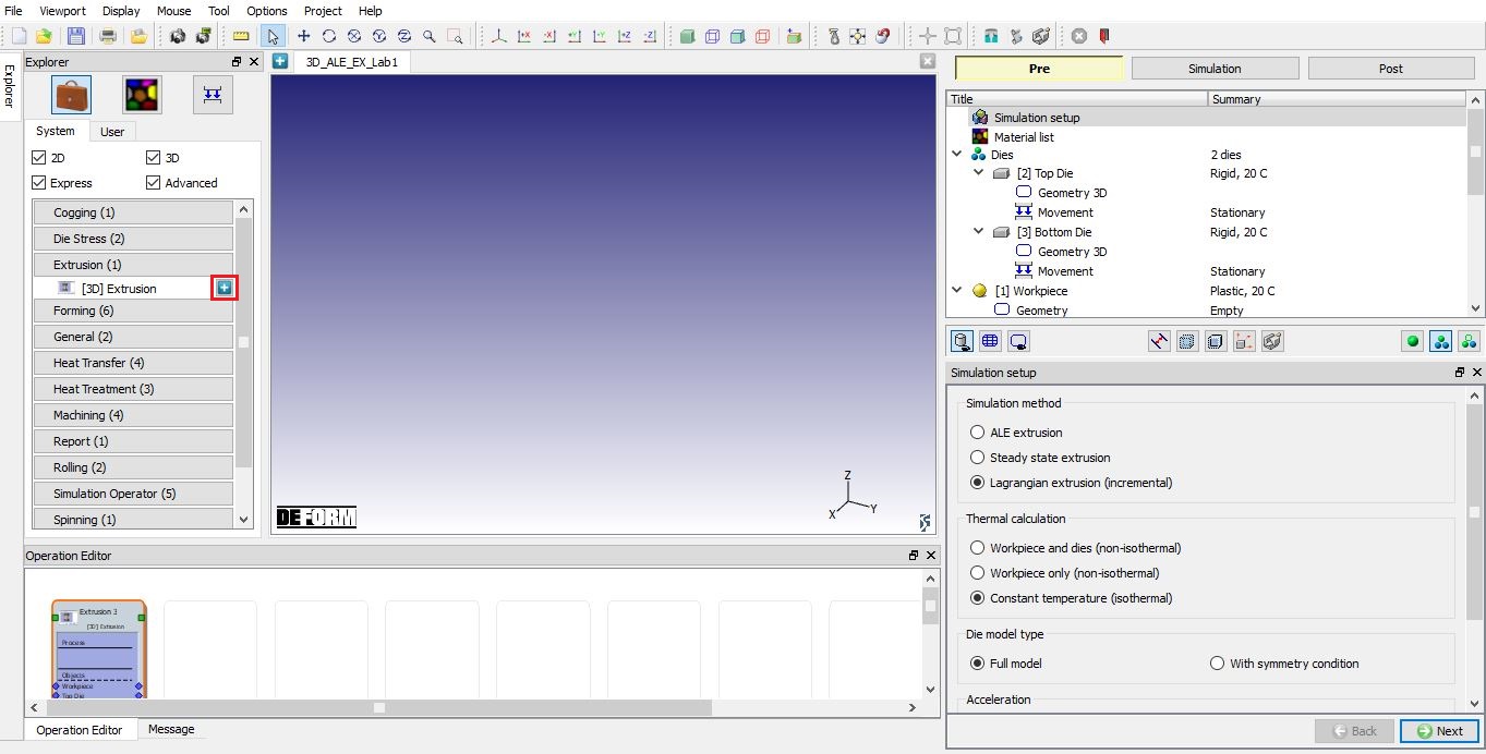
Add 3D Extrusion operation from the Explorer Operations list. Add the operation by clicking on ![]() button available next to 3D Extrusion or can also be added by drag and drop into the Operation editor (see Fig. ALEEXL1.4.). When we add the Extrusion operation, process settings Window will open by default.
button available next to 3D Extrusion or can also be added by drag and drop into the Operation editor (see Fig. ALEEXL1.4.). When we add the Extrusion operation, process settings Window will open by default.
Adding 3D Extrusion operation
Simulation Setup
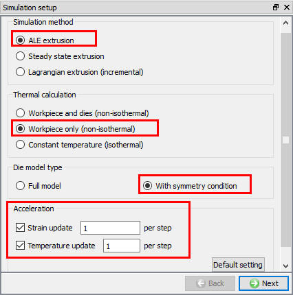
In the Simulation setup dialog, choose ALE extrusion radio button as Simulation method. Set Thermal calculation asWorkpiece only (non–isothermal) and Die model type as With symmetry condition. select both Strain update and Temperature update and set the value with1 per step in Acceleration, which means there is no acceleration updating in this simulation. Simulation setup looks like as shown as Fig. ALEEXL1.5. Then click ![]() to Material list page.
to Material list page.
Simulation setup settings
Material list
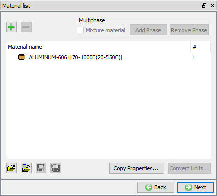
In the Material dialog, click Load material data from library ![]() . Load the material ‘ALUMINUM-6061[70-1000F(20-550C)] ‘ from Aluminum category, as shown in Fig. ALEEXL1.6., and then click
. Load the material ‘ALUMINUM-6061[70-1000F(20-550C)] ‘ from Aluminum category, as shown in Fig. ALEEXL1.6., and then click ![]() to Dies page.
to Dies page.
Material list
Dies
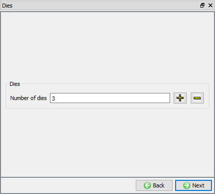
By Default, 2 dies will be added in operation, in this lab we need 3 dies. So, click on ![]() button to make Number of Dies as 3 (see Fig. ALEEXL1.7.). Click on
button to make Number of Dies as 3 (see Fig. ALEEXL1.7.). Click on ![]() to Top Die page.
to Top Die page.
Added Dies
Ram
Change the name of the Top Die object to Ram. Set the die temperature to 400 °C and keep the object type to Rigid and uncheck the Assign Bearing surface check box. Then click on ![]() to Geometry page.
to Geometry page.
Ram Geometry
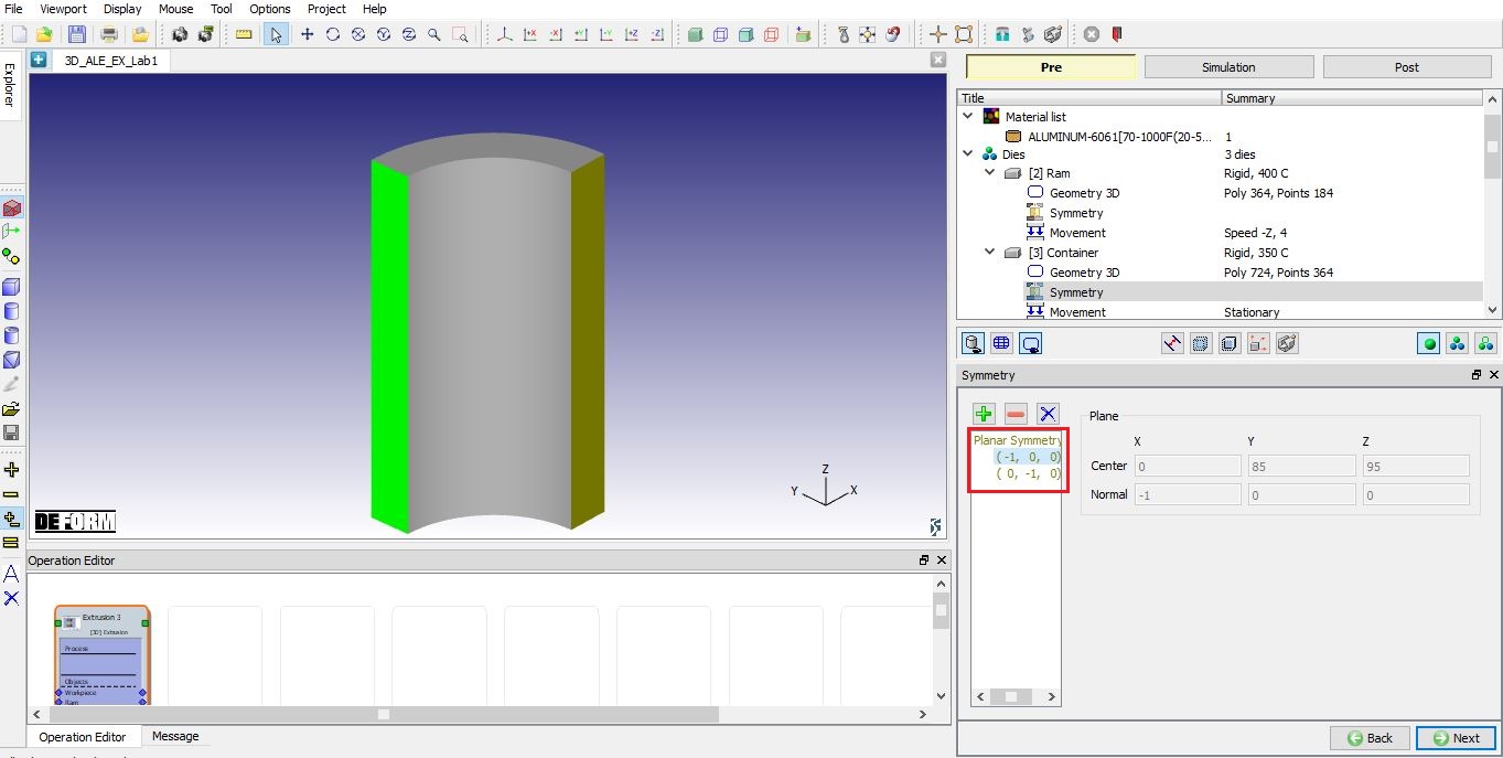
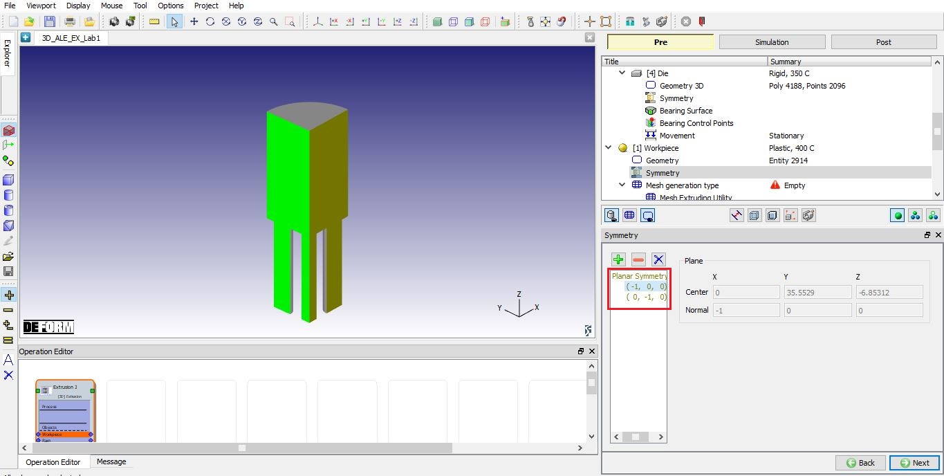
Click on Import geometry from library ![]() and load Ram_Geo.stl from 3D/LABS folder, then click
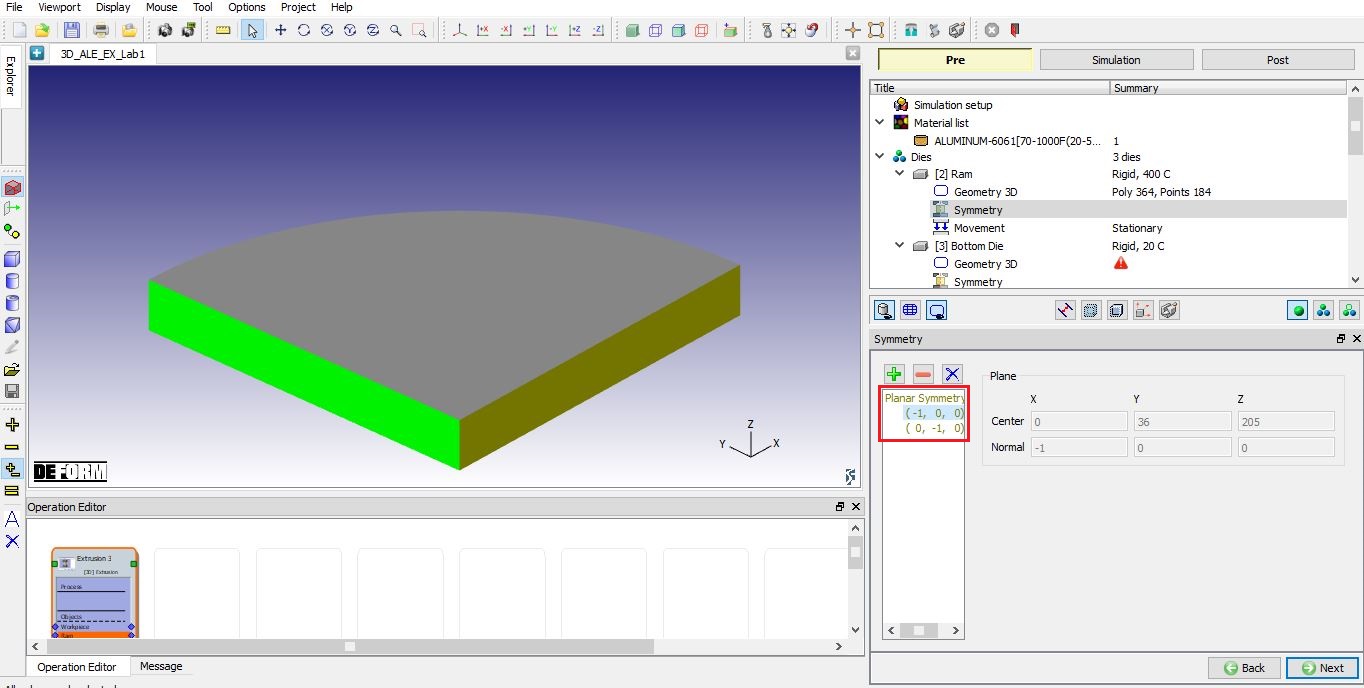
and load Ram_Geo.stl from 3D/LABS folder, then click ![]() to Symmetry page. In Symmetry dialog, define Planar Symmetry for the Ram on Symmetry planes as shown in (see Fig. ALEEXL1.8.). Click
to Symmetry page. In Symmetry dialog, define Planar Symmetry for the Ram on Symmetry planes as shown in (see Fig. ALEEXL1.8.). Click ![]() to Movement page.
to Movement page.
Ram Geometry
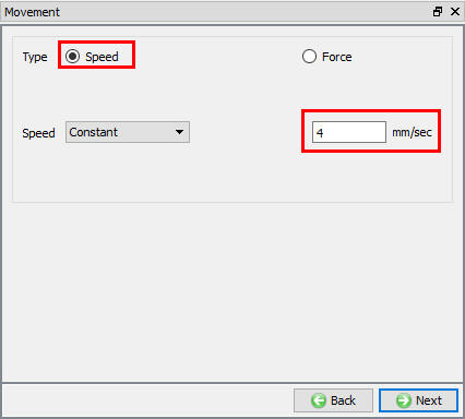
Ram Movement
In the Movementdialog , define the Speed as 4 mm/sec as shown in Fig. ALEEXL1.9. Click ![]() to Bottom Die page.
to Bottom Die page.
Ram Movement page
Container
Change the name of the Bottom die to Container. Set the die temperature to 350 °C and keep the object type to Rigid and uncheck the Assign Bearing surface check box. Then click on ![]() to Geometry page.
to Geometry page.
Container Geometry
Click on Import geometry from library ![]() and load Container_Geo.stl file from 3D/LABS folder, then click on
and load Container_Geo.stl file from 3D/LABS folder, then click on ![]() . In Symmetry dialog, define Planar Symmetry for the Container on Symmetry planes as shown in Fig. ALEEXL1.10. Click on
. In Symmetry dialog, define Planar Symmetry for the Container on Symmetry planes as shown in Fig. ALEEXL1.10. Click on ![]() to Movement page.
to Movement page.
Container geometry
Container Movement
In the Movement dialog, leave the Speed as 0 mm/sec. Click on ![]() to Object 4 page.
to Object 4 page.
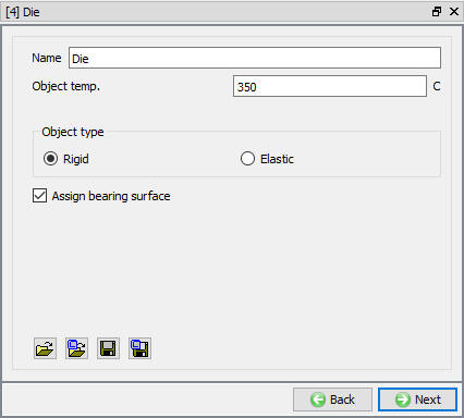
Die
Change the name of the Object 4 to Die. Set the die temperature to 350 °C. Keep the object type to Rigid and checkAssign Bearing Surface for ALE extrusion (see Fig. ALEEXL1.11.). Then click on ![]() to Geometry page.
to Geometry page.
Setting of the Die
Die Geometry
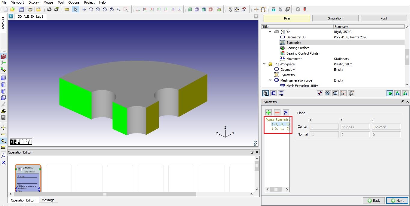
Click Import geometry from library ![]() and load Die_Geo.stl file from 3D/LABS folder, then click on
and load Die_Geo.stl file from 3D/LABS folder, then click on ![]() . In Symmetry dialog, define Planar Symmetry for the Die on Symmetry planes as shown in Fig. ALEEXL1.12. Click on
. In Symmetry dialog, define Planar Symmetry for the Die on Symmetry planes as shown in Fig. ALEEXL1.12. Click on ![]() to Bearing Surface page.
to Bearing Surface page.
Die geometry
Bearing Surface
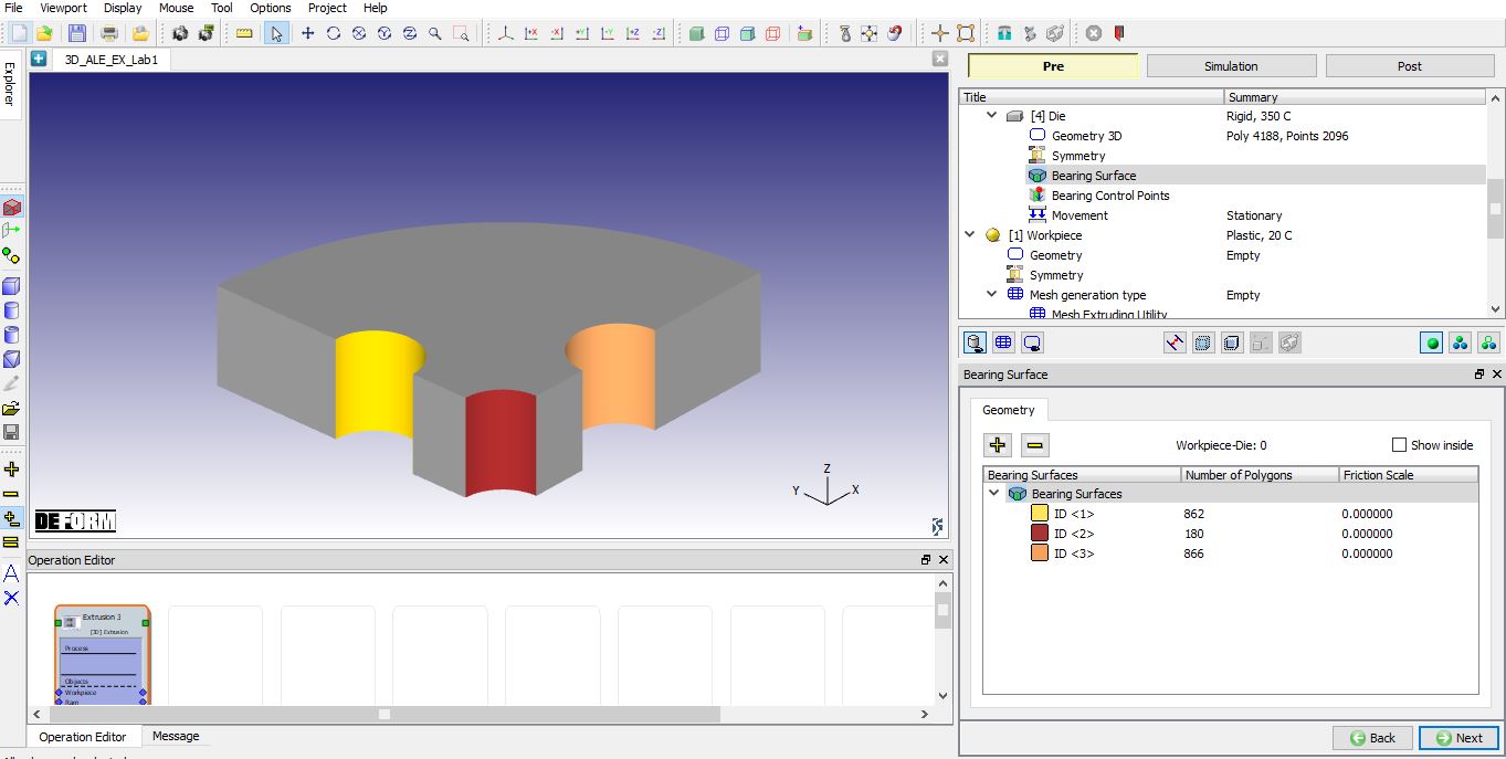
In Bearing Surface page, we will define bearing surfaces and add them to the bearing surface list. For this die object, there are 3 bearing surfaces. Keep the Select mode in the left column. To define the bearing surface, we select all the patches related to the bearing and click ![]() button. A highlighted bearing surface withID <1> will be added to the list when we defined the first bearing surface. Then we define the second and the third bearing surfaces similarly. Complete list of bearing surfaces is shown in Fig. ALEEXL1.13. The first, second and third bearing surfaces are highlighted with yellow, red and orange color respectively in the die geometry display. Click on
button. A highlighted bearing surface withID <1> will be added to the list when we defined the first bearing surface. Then we define the second and the third bearing surfaces similarly. Complete list of bearing surfaces is shown in Fig. ALEEXL1.13. The first, second and third bearing surfaces are highlighted with yellow, red and orange color respectively in the die geometry display. Click on ![]() to go to Bearing Control Points page.
to go to Bearing Control Points page.
Bearing Surface
Bearing Control points
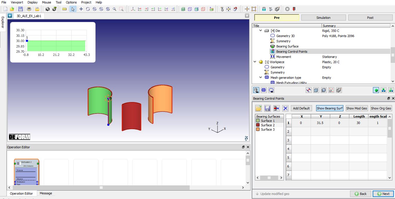
After define the bearing surface, a virtual bearing and it bearing length distribution will be generated for bearing control points definition (see Fig. ALEEXL1.14.). In “3D_SS_EX_Lab1 “, we will introduce how to define bearing control points to adjust the bearing length. In this lab, we will not adjust the bearing length, so there is no need to define bearing control points. Click on ![]() to movement page.
to movement page.
Bearing surface original settings
Die Movement
In the Movement dialog, leave the Speed as 0 mm/sec. Go to next page by clicking ![]() button .
button .
Workpiece
Keep the default name of the Workpiece object as Workpiece. Set the Workpiece temperature to 400 °C and keep the object type as Plastic. Click on ![]() to Geometry page.
to Geometry page.
Workpiece geometry
Click Import geometry from library ![]() and load ALE_Workpiece_Geo.stl from 3D/LABS folder, then click
and load ALE_Workpiece_Geo.stl from 3D/LABS folder, then click ![]() . In Symmetry dialog, definePlanar Symmetry for the workpiece on Symmetryplanes as shown in (see Fig. ALEEXL1.15.). In this lab, the length of extrudate is 120 mm, the length in container is 150 mm. Click on
. In Symmetry dialog, definePlanar Symmetry for the workpiece on Symmetryplanes as shown in (see Fig. ALEEXL1.15.). In this lab, the length of extrudate is 120 mm, the length in container is 150 mm. Click on ![]() to Mesh generation type page.
to Mesh generation type page.
Workpiece geometry
Workpiece Mesh Generation type
In the Mesh Generation Type page, two options are provided for mesh generation of ALE workpiece. One is Mesh Extruding Utility and the other is Regular Meshing.
In the previous versions for ALE and Steady state extrusion simulations, mesh was generated using Regular Meshing (DEFORM-3D mesh generator). The mesh generator first creates a surface mesh and then generates an unstructured tetrahedral volumetric mesh.
In this lab, we will demonstrate how to generate extruded mesh using Mesh Extruding Utility.
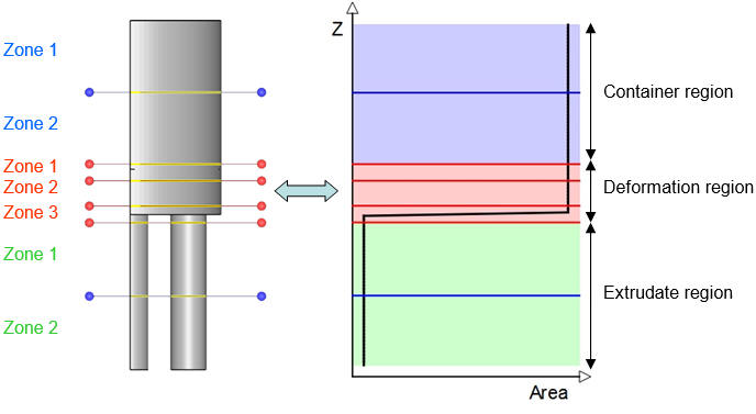
In simulations of ALE and Steady state extrusion, we can consider the workpiece consisting of three different regions: container region, extrudate region and deforming region. The container region and extrudate region are simple extruded shapes, while the deforming region is much more complex.
The Mesh Extruding Utility allows users to mesh only the complex deforming region using DEFORM-3D mesh generator firstly. Then, extruded mesh of the container region and the extrudate region can be generated by adding layers of elements in those areas.
ChooseMesh Extruding Utility and click ![]() . The system will give a template for mesh generation of three regions.
. The system will give a template for mesh generation of three regions.
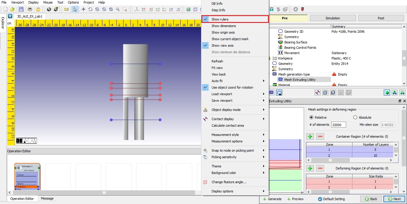
Using right click menu options from the display area select “Show rulers “ as shown in Fig. ALEEXL1.16. to display ruler which will help us in placing the different regions.
The default setting of the three regions are based on the cross-section areas of the workpiece along the Z direction. The region division is shown as Fig. ALEEXL1.17.
Mesh Extruding Utility
Region division
In this lab, we will adjust the parameters in the Mesh Extruding Utility.
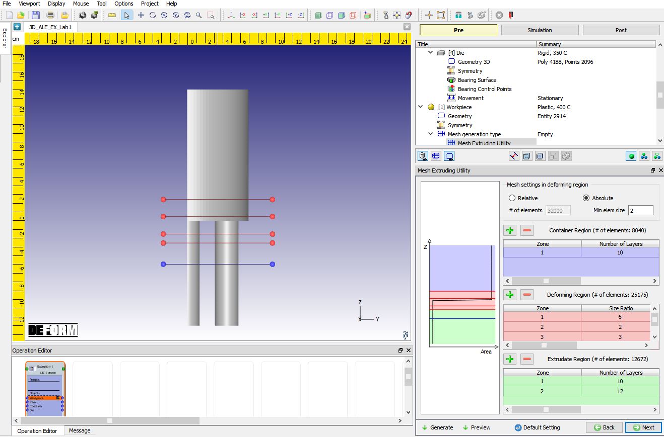
Firstly, we will adjust the deformation region. The deformation region (subdomain) between the top red line and the bottom red line will be used to generate regular mesh with DEFORM-3D mesh generator. So, we can use the regular method to define the mesh density which is similar to Mesh Window setting.
Keep 3 zones and drag the zone lines to our expected positions. Approximately drag the top red line to Z = 25 mm, the second red line to Z = 5 mm, the third red line to Z = -15 mm, the bottom red line to Z = -25 mm.
Zone 1 will define the mesh density near container region. Zone 2 will define the mesh density near bearing entry. Zone 3 will define mesh density near extrudate region. In Mesh setting in deformation region dialog, select ‘Absolute ‘ Type and set Min elem size with ‘2 mm’. In the table of Deformation Region, set Element Size of Zone 1 with ‘6 mm’, Zone 2 with ‘2 mm’ and Zone 3 with ‘3 mm’. If the deformation region is much more complex, we should add zones by clicking ‘ ![]() ’ and define their suitable mesh densities.
’ and define their suitable mesh densities.
Then in Container Region, delete 1 zone by clicking ‘![]() ’. Set Number of layers with ‘10’ in Zone 1.
’. Set Number of layers with ‘10’ in Zone 1.
In Extrudate Region, keep 2 zones and drag the zone line (blue line) to Z = -50 mm. Set Number of layers with ‘10’ in Zone 1, and with ‘12’ in Zone 2.
The adjusted parameters settings in Mesh Extruding Utility is shown as Fig. ALEEXL1.18.
Parameters settings for Mesh Extruding Utility
In Fig. ALEEXL1.18., we can see three buttons at the bottom of the widget – Default Setting , Preview and Generate. Default Setting will reset all the mesh parameters to the default setting. Preview will create a subdomain geometry and generate surface mesh for the deforming region. Generate will generate solid mesh for the deforming region and add layered elements in the container and extrudate regions. If Preview is not clicked previously, Generate will complete all the tasks consecutively.
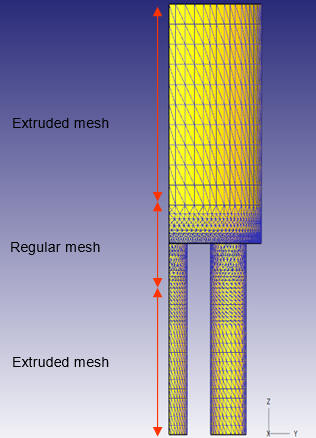
Click on Generate to generate the mesh of the workpiece. The generated workpiece mesh is shown in Fig. ALEEXL1.19. We can clearly see the regular mesh in deformation region and extruded mesh in container & extrudate regions. Click on ![]() to Material page.
to Material page.
Workpiece mesh generated
Workpiece Material
Assign ALUMINUM-6061[70-1000F(20-550C)] as the material for Workpiece, click on ![]() to Boundary condition page.
to Boundary condition page.
Workpiece Boundary condition
The system automatically assigned the symmetry plane BCC to the workpiece after mesh generation (see Fig. ALEEXL1.20.).
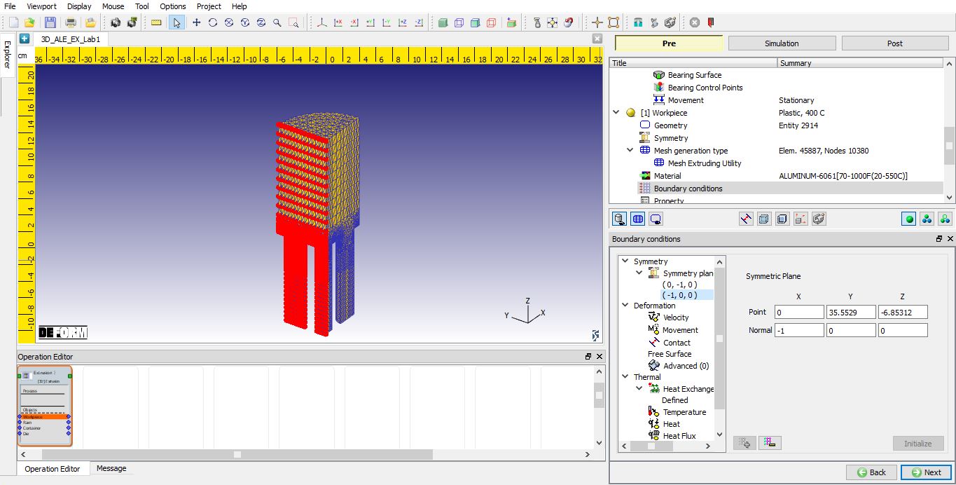
Symmetry BCC of the Workpiece
For ALE and Steady state extrusion, a Free Surface needs to be defined at the end of the extrudate. In the Boundary conditions dialog, click FreeSurface in the tree, rotate the workpiece so that you can see the bottom of the extrudate, select the bottom surface and then Click ![]() to add the Free surface boundary condition (see Fig. ALEEXL1.21.).
to add the Free surface boundary condition (see Fig. ALEEXL1.21.).
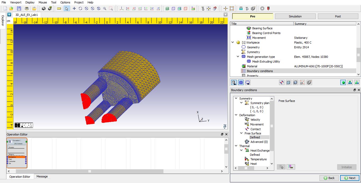
Free Surface BCC of the Workpiece
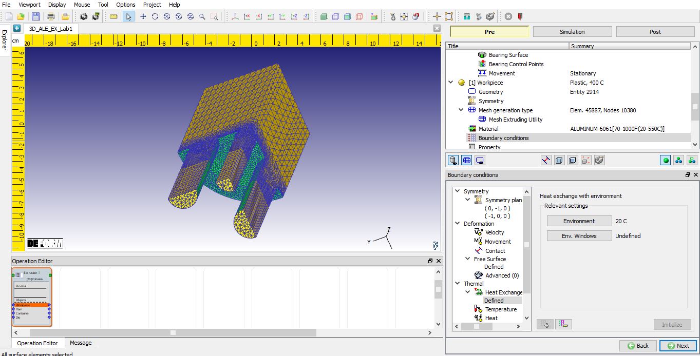
The system automatically assigned Heat Exchange with Environment BCC to the workpiece after mesh generation. For ALE & Steady state extrusion, Free Surface should not be assigned with Heat Exchange with Environment BCC hence, we should delete the existing Heat Exchange with Environment BCC on the free surface by clicking on ‘Defined ‘ and ![]() . We redefine the Heat Exchange with Environment BCC. In the left pick bar, click the
. We redefine the Heat Exchange with Environment BCC. In the left pick bar, click the ![]() button to select all the surfaces, then click and click the Free Surface & symmetry surfaces to unselect them. Click
button to select all the surfaces, then click and click the Free Surface & symmetry surfaces to unselect them. Click ![]() to add the Heat Exchange with Environment BCC. Defined Heat Exchange with Environment BCC is as shown in Fig. ALEEXL1.22. Click
to add the Heat Exchange with Environment BCC. Defined Heat Exchange with Environment BCC is as shown in Fig. ALEEXL1.22. Click ![]() until Control page.
until Control page.
Heat Exchange with Environment BCC of the Workpiece
Controls
In the Control page. we can use ![]() to adjust the positions of objects.
to adjust the positions of objects.
All the die components were imported from the .stl files. The container and the die were in the correct locations. The ram is away from the workpiece. Hence, we need to move the ram down to touch the workpiece.
Click ![]() and specify
and specify ![]() positioning. Select the Ram as the Positioning object and the Workpiece as the Reference. Verify that the Approach direction is–Z. Click on
positioning. Select the Ram as the Positioning object and the Workpiece as the Reference. Verify that the Approach direction is–Z. Click on ![]() and then
and then ![]() . Click on
. Click on ![]() to Contact page.
to Contact page.
Contact
A message will pop-up (see Fig. ALEEXL1.23.) as we enter the Inter-object relations page and ask if user wants to use special contact generation algorithm to generate full contact. Click ![]() .
.
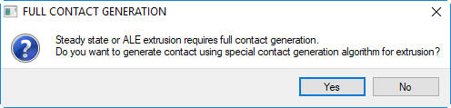
FULL CONTACT GENERATION popup
In the Contact page, click ![]() to create all the relationships of the workpiece with other objects. Then click on
to create all the relationships of the workpiece with other objects. Then click on ![]() to generate full contact of the workpiece with other objects. Then, let’s edit the parameters setting for contact relationships of the workpiece.
to generate full contact of the workpiece with other objects. Then, let’s edit the parameters setting for contact relationships of the workpiece.
Select the Ram – Workpiece relationship and click ![]() . Define contact separation as ‘Non-separable ‘, Shear friction as ‘1.0 ‘ and heat transfer coefficient as’11.0 ‘.
. Define contact separation as ‘Non-separable ‘, Shear friction as ‘1.0 ‘ and heat transfer coefficient as’11.0 ‘.
Select the Container – Workpiece relationship and click ![]() . Define contact separation as ‘Non-separable ‘, Shear friction as’1.0 ‘ and heat transfer coefficient as’11.0 ‘.
. Define contact separation as ‘Non-separable ‘, Shear friction as’1.0 ‘ and heat transfer coefficient as’11.0 ‘.
Select the Die – Workpiece relationship and click ![]() . Define contact separation as ‘Non-separable ‘, Shear friction as ‘0.4 ‘ and heat transfer coefficient as ‘11.0 ‘ (See Fig. ALEEXL1.24.). Click on
. Define contact separation as ‘Non-separable ‘, Shear friction as ‘0.4 ‘ and heat transfer coefficient as ‘11.0 ‘ (See Fig. ALEEXL1.24.). Click on ![]() to Step controls.
to Step controls.
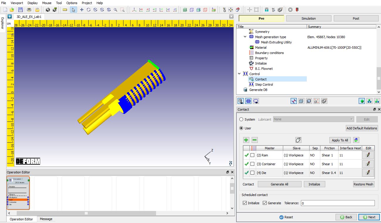
Full contact generation of the workpiece
Step Controls
Click ‘![]() ‘ to switch to expert mode in the top menu bar for step control.
‘ to switch to expert mode in the top menu bar for step control.
Simulation steps
In the Simulation steps ![]() dialog, set Number of simulation steps as ‘2000 ‘ and StepIncrementtosave as ‘100 ‘. SetPrimary die as ‘2 - Ram ‘ (see Fig. ALEEXL1.25.).
dialog, set Number of simulation steps as ‘2000 ‘ and StepIncrementtosave as ‘100 ‘. SetPrimary die as ‘2 - Ram ‘ (see Fig. ALEEXL1.25.).
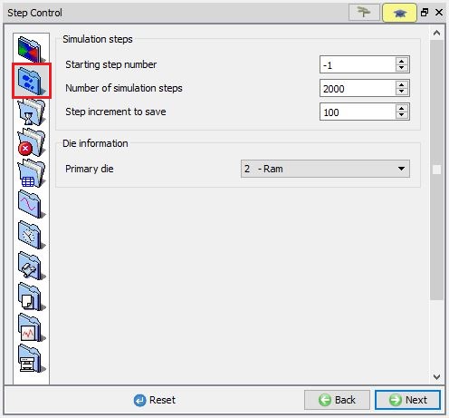
Simulation step Setup
In ALE extrusion simulation, since there is no gap between the workpiece and the container, we can use constant step increment. But in ALE extrusion simulation, we must consider the limitations of the minimum element size and the workpiece dimensions to set the time step setting.
-
In this lab, the minimum element size is 2 mm. From the “3D_Lagrangian_EX_Lab1”, the movement velocity of the extrudate is 21.16 mm/s, so the appropriate time/step of the ram would be 0.03 sec/step.
-
The material should at least flow out the entire extrudate. In this lab, the length of extrudate is 120 mm, the minimum time for the material to flow out the free surface (the end of the extrudate) is 5.67 (120/21.16) s. If we want to simulation 2000 steps, the minimum time step increment should be 0.00284 sec/step.
-
The material cannot flow out of the container completely. In this lab, the length in container is 150 mm, the movement velocity of the ram is 4 mm/s, the maximum time for the material to flow out of the container completely is 37.5 (150/4) s. If we want to simulation 2000 steps, the maximum time step increment should be 0.01875 sec/step.
Base on above three aspects, we can select 0.01 sec/step as the step increment. In the Stepincrement![]() **dialog, set Solution step definition as **Time. Set Step increment control to Constant and define it as ‘0.01 ‘ sec/step (see Fig. ALEEXL1.26.).
**dialog, set Solution step definition as **Time. Set Step increment control to Constant and define it as ‘0.01 ‘ sec/step (see Fig. ALEEXL1.26.).
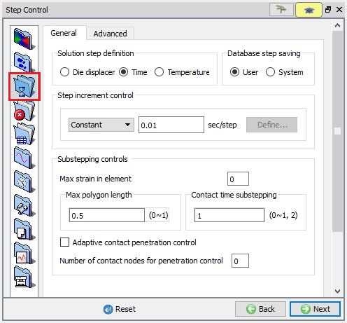
Step increment setup
Stop criteria
In the Stop criteria![]() dialog, click the ALESteadyState page, uncheck ‘Turn on steady-state stop control ‘ if not unchecked (see Fig. ALEEXL1.27.).
dialog, click the ALESteadyState page, uncheck ‘Turn on steady-state stop control ‘ if not unchecked (see Fig. ALEEXL1.27.).
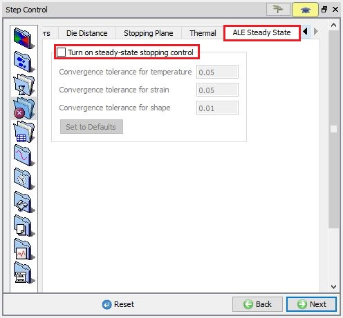
Stopping control
Double constraints settings
For ALE and Steady state extrusion, the system will generate double constraints automatically in simulation.
Generate DB
Then go to Generate DB page. Click ![]() to see if anything was missed in the setup and then click on the
to see if anything was missed in the setup and then click on the ![]() button to generate the database. Observe the message in Message tab informing database generation status.
button to generate the database. Observe the message in Message tab informing database generation status.
Running Simulation
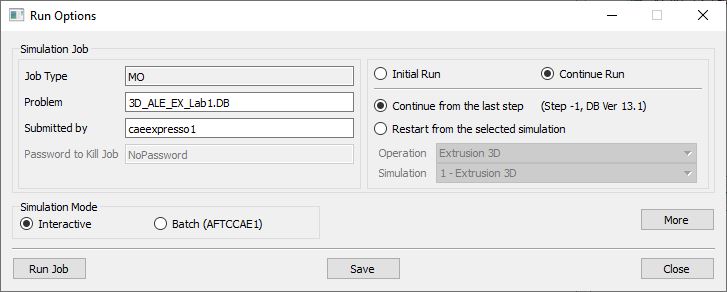
Once the database has been generated switch to the Simulation mode by clicking on ![]() button above the operation tree. Click on the
button above the operation tree. Click on the ![]() action label to open the Run Options dialog as shown in Fig. ALEEXL1.28.Use the default ContinueRun option to select “Continue from the last step ” (from step -1) option and then select the Simulation mode as Interactive radio button. Click on
action label to open the Run Options dialog as shown in Fig. ALEEXL1.28.Use the default ContinueRun option to select “Continue from the last step ” (from step -1) option and then select the Simulation mode as Interactive radio button. Click on ![]() button to run the simulation.
button to run the simulation.
To define MPI settings, click on ![]() button, Run Options window will expand and displays options to define MPI settings for simulation (max number of processors that can be defined depend on your 3D MPI license).
button, Run Options window will expand and displays options to define MPI settings for simulation (max number of processors that can be defined depend on your 3D MPI license).
Run Simulation Window
Monitor the progress of the simulation by looking at the Simulation Message and Simulation Log tab, make sure that the ![]() option is checked. User can view the Extrusion process from simulation graphics as the simulation proceeds to the specified Step definition.
option is checked. User can view the Extrusion process from simulation graphics as the simulation proceeds to the specified Step definition.
Acceleration Updating of State Variables
After above simulation is completed, save the project by clicking ![]() in the extrusion template. We should keep the simulation set up and simulation result of this project and do the simulation of acceleration with another project.
in the extrusion template. We should keep the simulation set up and simulation result of this project and do the simulation of acceleration with another project.
Simulation step up of Acceleration
In File menu ![]() click on New
click on New![]() and click on
and click on ![]() in both Question popups, new Project will be open with New project popup.
in both Question popups, new Project will be open with New project popup.
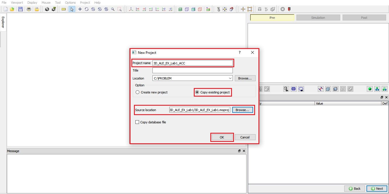
In New Project popup define the Project name as “3D_ALE_EX_Lab1_ACC “, select Copy existing project radio button, click on browse and browse “ 3D_ALE_EX_Lab1” project and click on ![]() in New Project popup as shown in Fig. ALEEXL1.29.
in New Project popup as shown in Fig. ALEEXL1.29.
New Project for Acceleration updating lab
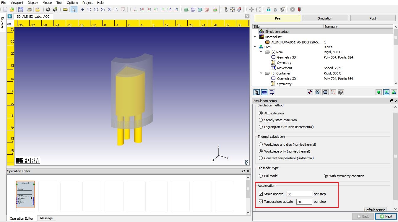
In the Simulation setup dialog, change both the Strainupdate and Temperatureupdate with50 per step in Acceleration, which means there will be 50 times acceleration updating in the next simulation. Keep other parameters settings untouched. Simulation setup is shown as Fig. ALEEXL1.30.
Simulation setup settings with State Variable update Acceleration
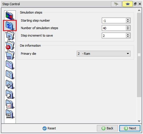
Go to StepControl page. In the Simulationsteps dialog, set Number of simulation steps as ‘40 ‘ and Step Increment to save as ‘2 ‘ (see Fig. ALEEXL1.31.).
Simulation steps for Acceleration
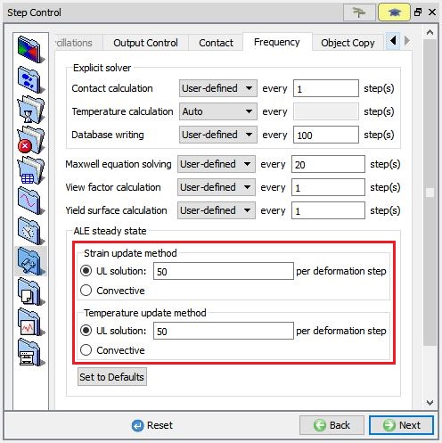
Check the defined acceleration setting is in Step Control page -> Advanced options dialog -> Frequency page (see Fig. ALEEXL1.32.).
Acceleration settings in Frequency
Then go to Generate DB page. Click ![]() to see if anything was missed in the setup and then click on the
to see if anything was missed in the setup and then click on the ![]() button to generate the database. Observe the message in Message tab informing database generation status.
button to generate the database. Observe the message in Message tab informing database generation status.
Running Simulation
Once the database has been generated, switch to the Simulation mode by selecting the ![]() button above the object tree. Click on the
button above the object tree. Click on the ![]() action label to open the Run Options dialog as shown in Fig. ALEEXL1.28.Use the default ContinueRun option to select “Continue from the last step ” (from step -1) option and then select the Simulation mode as Interactive radio button. Click on
action label to open the Run Options dialog as shown in Fig. ALEEXL1.28.Use the default ContinueRun option to select “Continue from the last step ” (from step -1) option and then select the Simulation mode as Interactive radio button. Click on ![]() button to run the simulation.
button to run the simulation.
Post Processing
After the simulation of Extrusion process with acceleration of state variable update is completed, we can compare the simulation results in Post processor.
In DEFORM GUI Main window, highlight “3D_ALE_EX_Lab1.DB”, then click ![]() to open “3D_ALE_EX_Lab1.DB “ in DEFORM Post processor.
to open “3D_ALE_EX_Lab1.DB “ in DEFORM Post processor.
In DEFORM-2D/3D DEFORM Post, from the top menu bar, click File![]() Open , select “3D_ALE_EX_Lab1_ACC.DB “, then click
Open , select “3D_ALE_EX_Lab1_ACC.DB “, then click ![]() .
.
From the top menu bar, click Windows![]() **Tile Vertically** , we can see that both “3D_ALE_EX_Lab1.DB” and “3D_ALE_EX_Lab1_ACC.DB” are opened in DEFORM-2D/3D Post. Thus, we can compare the simulation results of 2 databases in the same display window.
**Tile Vertically** , we can see that both “3D_ALE_EX_Lab1.DB” and “3D_ALE_EX_Lab1_ACC.DB” are opened in DEFORM-2D/3D Post. Thus, we can compare the simulation results of 2 databases in the same display window.
For acceleration simulation, the effective step = simulation step * acceleration frequency. For example, in this lab, the acceleration frequency is 50, so the effective step is 1000 in simulation step 20, the effective step is 2000 in simulation step 40. The effective step of acceleration simulation corresponds to the simulation step of simulation without acceleration.
In the display window, with the right mouse, check both ‘DB Info ‘ and ‘Title ‘ to display the name of database and the simulation step.
Comparisons of Effective strain and Temperature of the workpiece at last step are given in Fig. ALEEXL1.33. and Fig. ALEEXL1.34. respectively. User can also compare the simulation results in other corresponding simulation steps.
From the comparisons of simulation results, we can see the state variables match very well in the corresponding simulation step. On the other hand, from the message files in this lab, the simulation time without acceleration is about 2 hours, the simulation time with acceleration is about 20 minutes. So, acceleration updating of state variables is a useful way to save simulation time in ALE extrusion simulation.
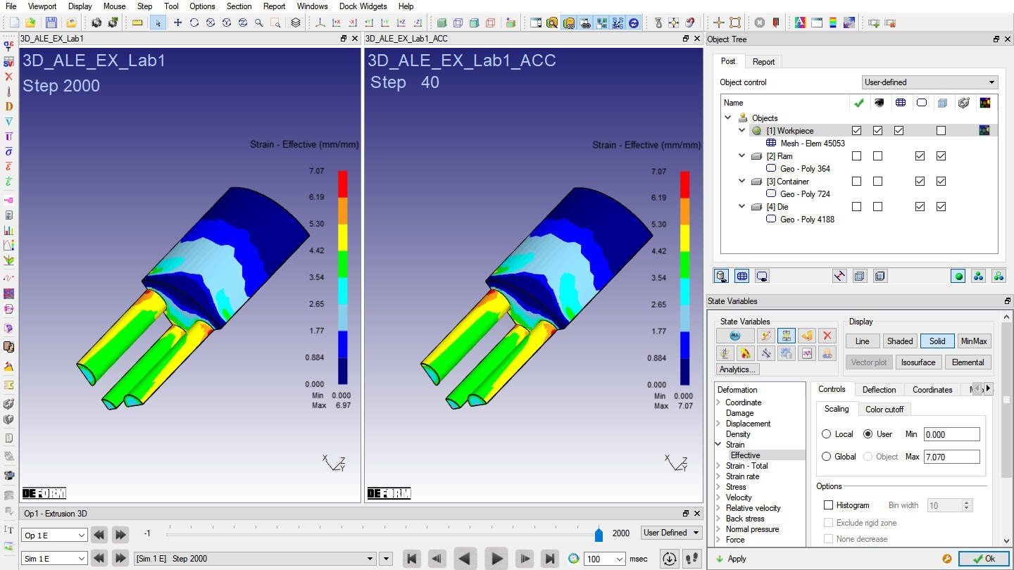
Strain Effective distribution at last step
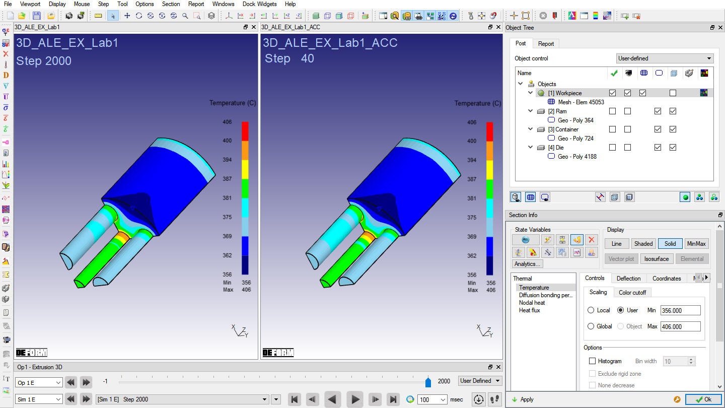
Temperature distribution at last step