Lagrangian Extrusion Lab1

In this Lab we are setting up a operation of Lagrangian extrusion.

The application of this lab will extrude 5 small cylinder parts from a large cylinder billet. The model of the workpiece is shown as Fig. LAGEXL1.1. The diameter of D0 is 140 mm. The diameter of D1 is 26 mm. The diameters of D2 and D4 are 27 mm. The diameters of D3 and D5 are 28 mm. Due to the model with symmetry, we will use a quarter model for simulation in this lab.

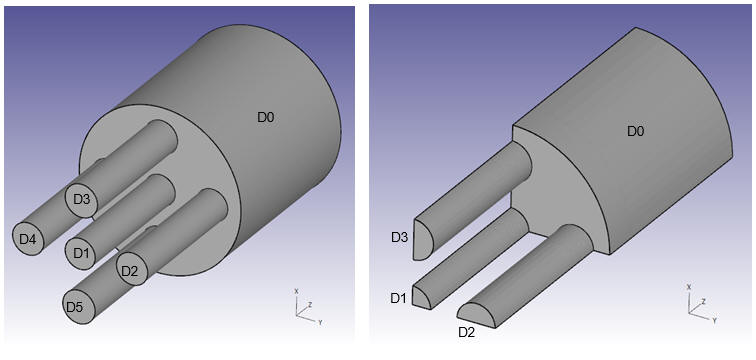
Model of the Workpiece

1.1. Creating a New Problem

1.2. Add Operation

1.3. Simulation Setup

1.4. Material list

1.5. Dies

1.6. Ram

1.7. Container

1.8. Die

1.9. Workpiece

1.10. Controls

1.11. Contact

1.12. Step Controls

1.13. Generate DB

1.14. Running Simulation

1.15. Post Processing

Creating a New Problem

On a Windows machine , go to the button select DEFORM-v1x.xxx (.xxx indicates version number E.g. v14.0.2) and select DEFORM GUI Main vxx.xx from the menu. The DEFORM GUI Main window will appear as shown below Fig. LAGEXL1.2.

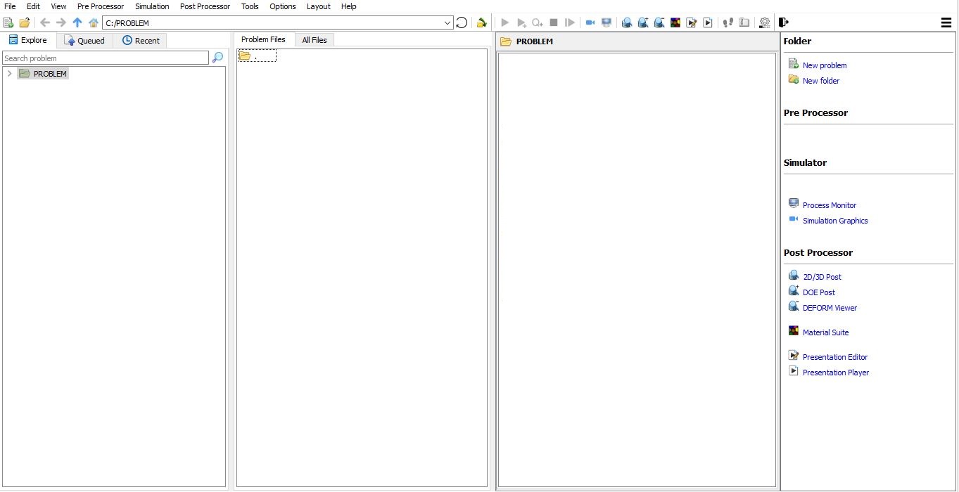
DEFORM GUI Main window

Create a new problem either by selecting File New Problem or by clicking the New Problem icon. The Problem Setup window will appear as shown in Fig. LAGEXL1.3. Select “Integrated Manufacturing Process “ radio button and unit system as “SI “ radio button in unit field. Define Problem Name as “**3D_Lagrangian_EX_Lab1** “ and make sure the “Show option dialog ” check box is turned on (if we do not turn on the “Show option dialog ” check box, then we will not get the New Project dialog in MO UI). Then click on button to open a new Problem using the Deform Integrated Manufacturing Process.

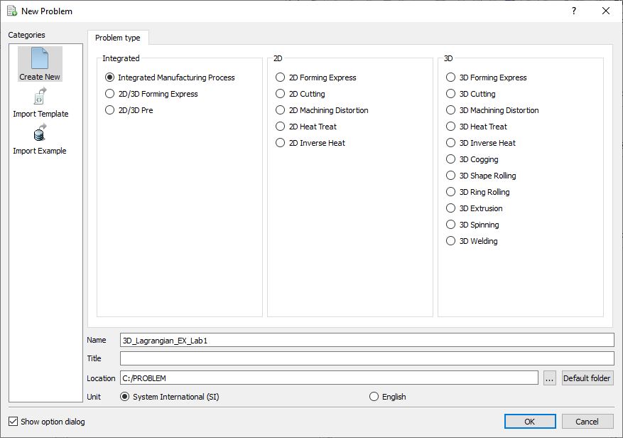
New Problem page

Multiple operation wizard will open with the New Project dialog, at this point user will be prompted to specify a project name (system will create a separate folder with this project name) and title for this session. In this session we will use “3D_Lagrangian_EX_Lab1 “ as the project name. Click on to continue to open the operation.

Adding Operation

Add 3D Extrusion operation from the Explorer Operations list. Add the operation by clicking on button available next to 3D Extrusion or user can also add by drag and drop into the Operation Editor (see Fig. LAGEXL1.4.). When we add the 3D Extrusion operation, process settings Window will open by default.

Adding Extrusion operation

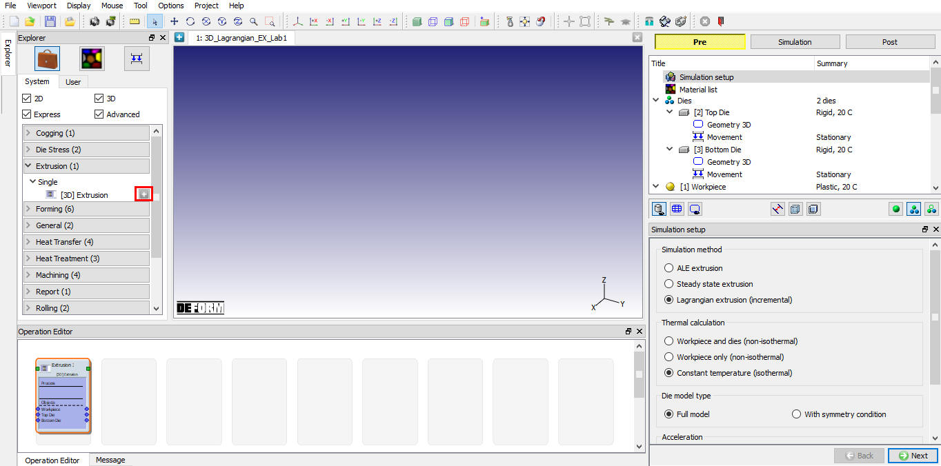
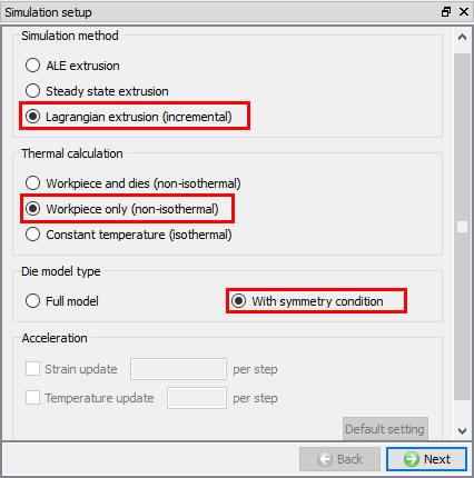
Simulation setup

In the Simulation Setup dialog, chooseLagrangian Extrusion (Incremental) radio button in Simulation Method. Set Thermal Calculation as Workpiece Only (Non – Isothermal) and Die Model Type as With symmetry condition. Simulation setup settings is shown in Fig. LAGEXL1.5. Click on to Material list page.

Simulation setup settings

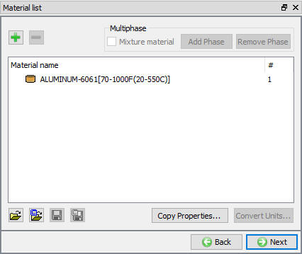
Material List

In the Material dialog, click Load material data from library . Load the material ‘ALUMINUM-6061[70-1000F(20-550C)] ‘ from Aluminum category, as shown in Fig. LAGEXL1.6., and then click on to Dies page.

.

Material list

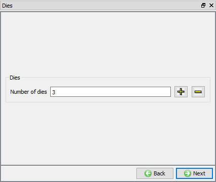
Dies

By Default, 2 dies will be added in operation, in this lab we need 3 dies. So, click on button to make Number of Dies as 3 (see Fig. LAGEXL1.7.). Click on to Top Die page.

Added Dies

Ram

Change the name of the Top Die object to Ram. Set the die temperature to 400 °C and keep the object type to Rigid. Then click on to Geometry page.

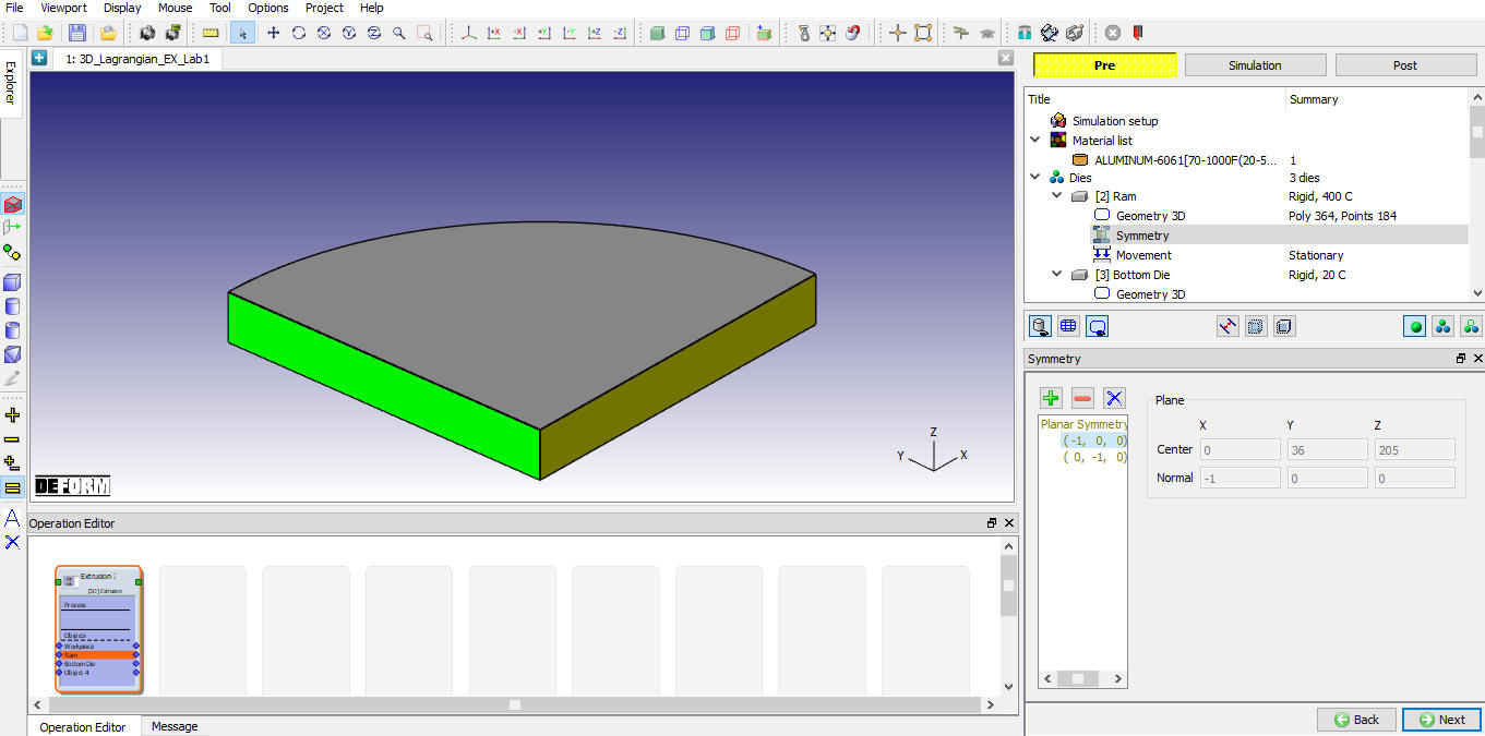
Ram Geometry

Click on Import geometry from library and load Ram_Geo.stl from 3D/LABS folder, then click on . In Symmetry dialog, define Planar Symmetry for the Ram on Symmetry planes as shown in (see Fig. LAGEXL1.8.). Click on to Movement page.

Ram Geometry

Ram Movement

In the Movement dialog, define the Speed as 4 mm/sec as shown in Fig. LAGEXL1.9. Click on to Bottom Die page.

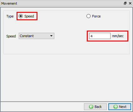
Ram Movement page

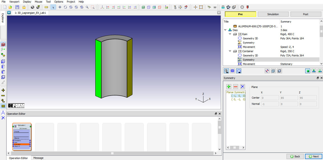
Container

Change the name of the Bottom die to Container. Set the die temperature to 350 °C and keep the object type to Rigid. Then click on to Geometry page.

Container Geometry

Click Import geometry from library and load Container_Geo.stl file from 3D/LABS folder, then click on . In Symmetry dialog, define Planar Symmetry for the Container on Symmetry planes as shown in Fig. LAGEXL1.10. Click on to Movement page.

Container Geometry

Container Movement

In the Movement dialog, leave the Speed as 0 mm/sec. Click on to Object 4 page.

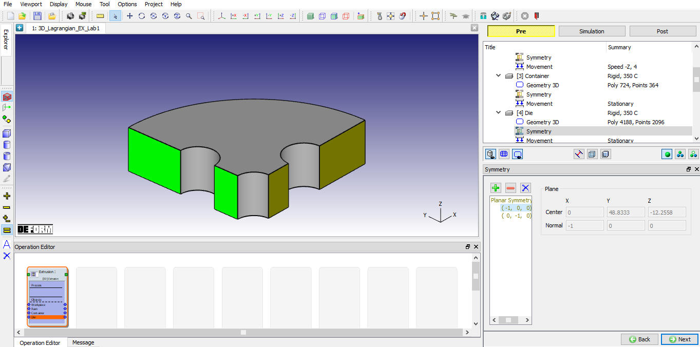
Die

Change the name of the Object 4 to Die. Set the die temperature to 350 °C and keep the object type to Rigid. Then click on to Geometry page.

Die Geometry

Click on Import geometry from library and load Die_Geo.stl file from 3D/LABS folder, then click on . In Symmetry dialog, define Planar Symmetry for the Die on Symmetry planes as shown in Fig. LAGEXL1.11. Click on to Movement page.

Die Geometry

Die Movement

In the Movement dialog, leave the Speed as 0 mm/sec. Go to Workpiece page by clicking .

Workpiece

Keep the default name of the workpiece object as Workpiece. Set the workpiece temperature to 400 °C and keep the object type to Plastic. Click on to Geometry page.

Workpiece geometry

The workpiece is a symmetrical cylinder, which can be easily created in DEFORM. Click on , select Cylinder and define a Height(H) as 178 mm and a Diameter(2R) as 138 mm. Define Startangle as 0 , RevolveAngle as 90 , Sections as 90. Click and . In Symmetry dialog, define Planar Symmetry for the workpiece on Symmetry planes as shown in (see Fig. LAGEXL1.12.). Click on to Mesh generation type page.

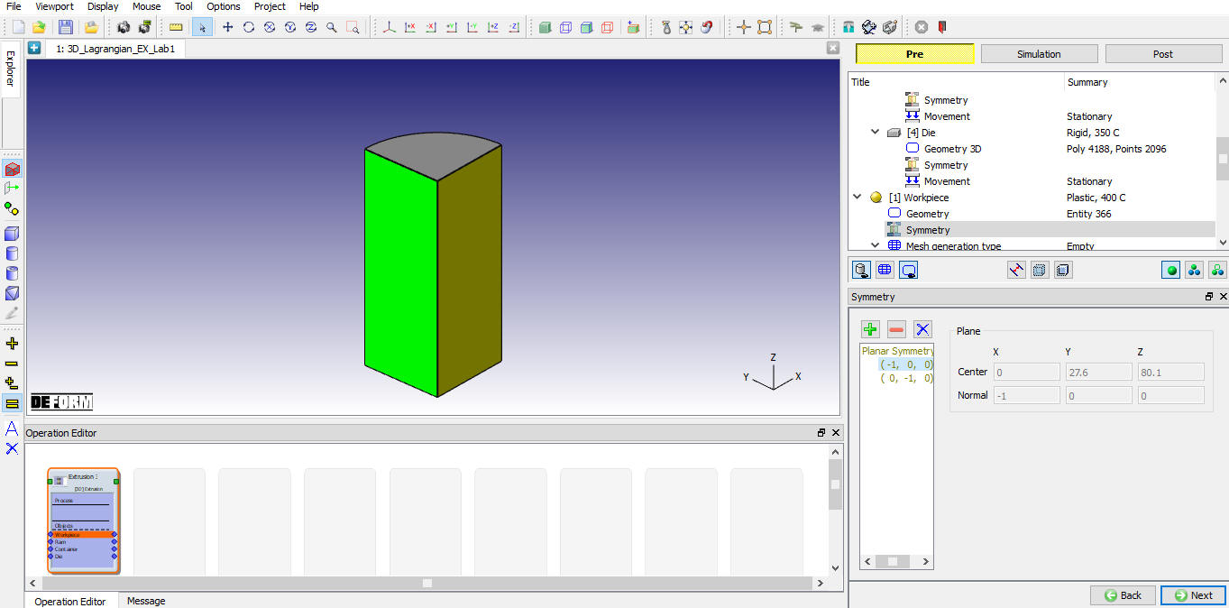
Workpiece Geometry

Workpiece Mesh

Generally, there are 2 rules for the mesh density setting for extrusion simulation. Firstly, there should be at least three elements throughout the thickness of the thinnest profile. At the same time, the mesh closed to the bearing zones should be finer than other places.

In the Mesh Generation Type page, two options are provided for meshing. One is Mesh Extruding Utility and the other is Regular Meshing. Choose Regular Meshing for Lagrangian extrusion. Then click on to Regular meshing page.

In General dialog, select ‘Absolute ‘ Type, set Sizeratio as ‘3 ‘ and Minimum elementsize as ‘2 mm’ as shown in Fig. LAGEXL1.13.

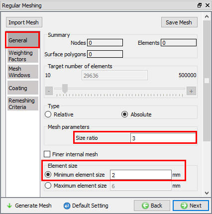
General Mesh page

In WeightingFactors dialog, set the factor of Mesh windows as ‘1.0 ‘ and otherfactors as ‘0.0 ‘ as shown in Fig. LAGEXL1.14.

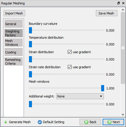
Workpiece Mesh -Weighting Factor page

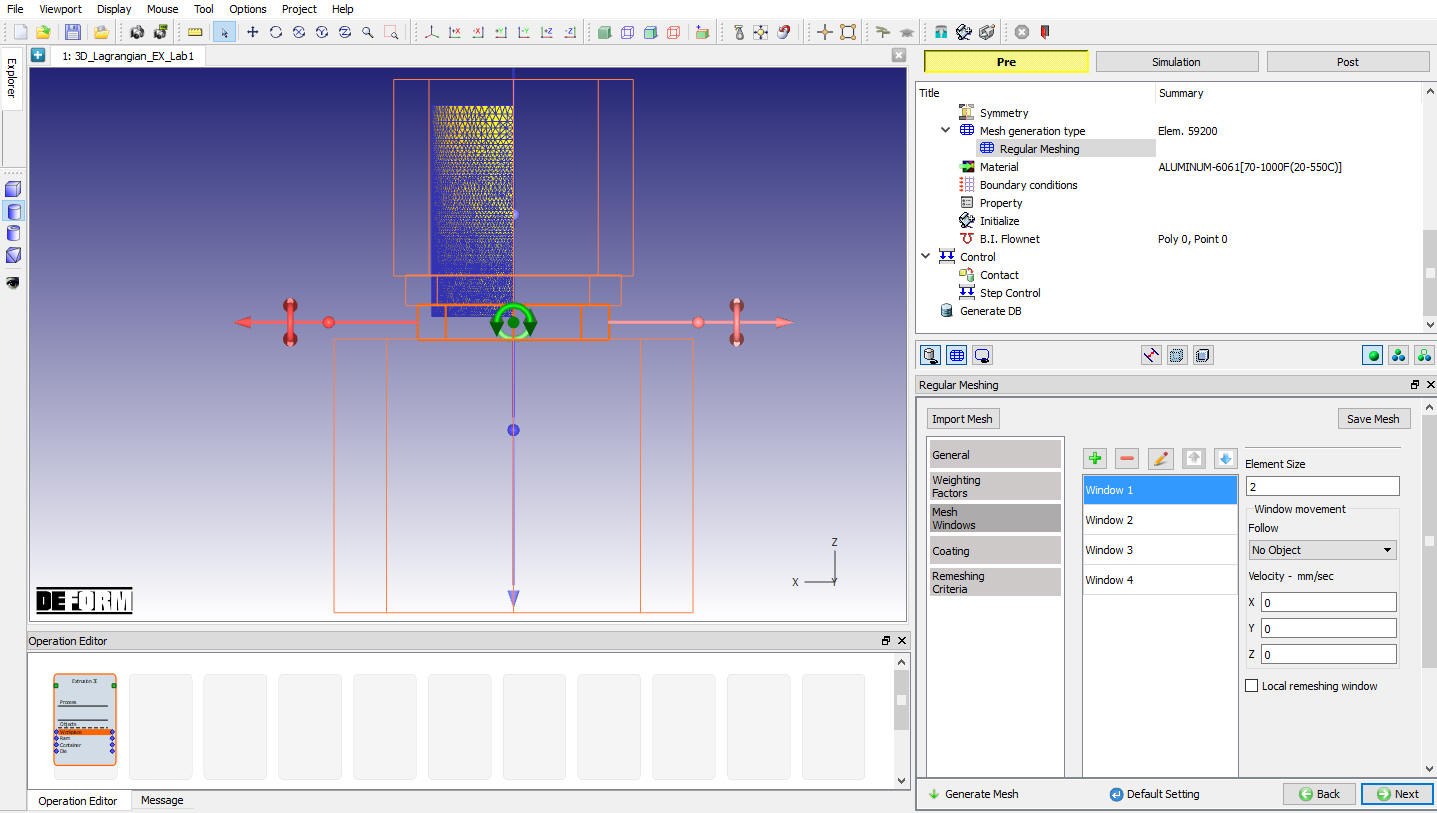
In Mesh Windows dialog, click Import Mesh Windows from a file and open UL_Workpiece_Mesh_Window.key from 3D/LABS folder.

Instead of importing the mesh windows, you can also create the mesh windows step by step.

1. On the Mesh Window tab, if there is any mesh window, click to delete all the existed mesh windows firstly.

2. On the Mesh Window tab, continuously click to create 4 mesh windows.

3. For each of these windows, click its name to highlight this window, then click cylinder window shape in the upper left Window Definition dialog , click on the screen in the workpiece to drop a cylinder mesh window into the Display window.

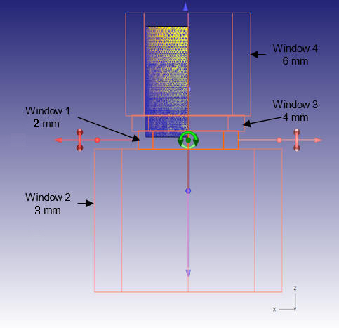
4. Click on to edit the dimension of each window. Edit the dimension of mesh Window 1, define Top Center as (0,0,10) and Bottom Center as (0,0,-20), define Radius as 80. Edit the dimension of mesh Window 2, define Top Center as (0,0,-19) and Bottom Center as (0,0,-250), define Radius as 150. Edit the dimension of mesh Window 3, define Top Center as (0,0,35) and Bottom Center as (0,0,9), define Radius as 90. Edit the dimension of mesh Window 4, define Top Center as (0,0,200) and Bottom Center as (0,0,34), define Radius as 100. Click after each edit.

5. Set the element size of mesh Window 1 with ‘2 mm’, the element size of mesh Window 2 with ‘3 mm’, the element size of mesh Window 3 with ‘4 mm’, and the element size of mesh Window 4 with ‘6 mm’.

In Lagrangian extrusion, the mesh windows will be used for the initial mesh generation and the remeshing during simulation. So, we must consider the material flow range during simulation and define correct mesh windows.

After defining the mesh windows, click on . Click in Default Boundary Conditions message dialog.

The mesh generation of the workpiece is shown in Fig. LAGEXL1.15. Click on to Material page.

Workpiece Mesh Windows page

Workpiece Material

Assign ALUMINUM-6061[70-1000F(20-550C)] as the material for Workpiece, click on to Boundary condition page.

Workpiece Boundary condition

The system automatically assigned the symmetry plane BCC to the workpiece after mesh generation (see Fig. LAGEXL1.16.).

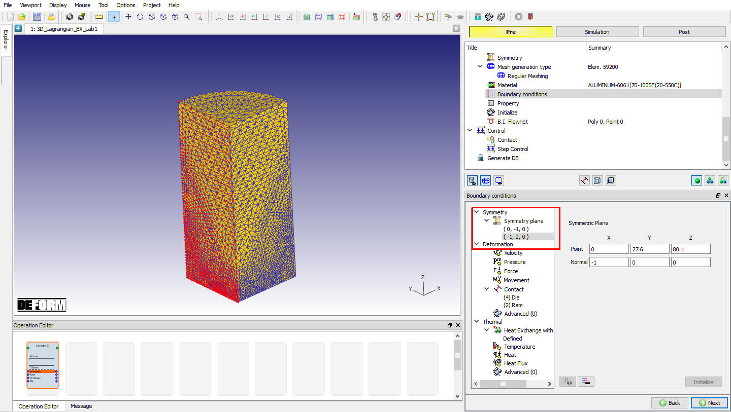
Symmetry BCC of Workpiece

The system automatically assigned Heat Exchange with Environment BCC to the workpiece after mesh generation. The result is shown in Fig. LAGEXL1.17. Click on until to Property page.

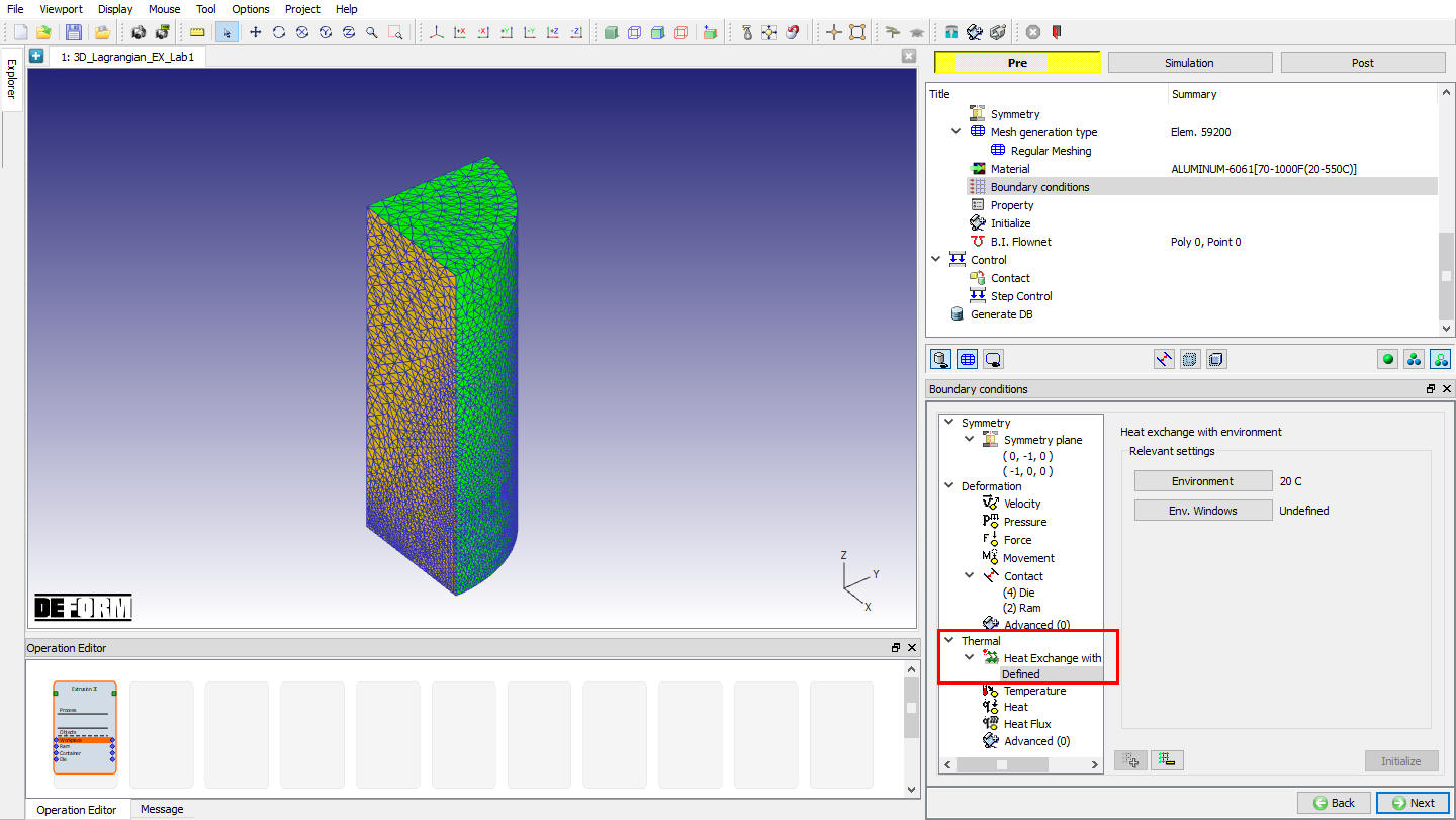
Thermal BCC of the workpiece

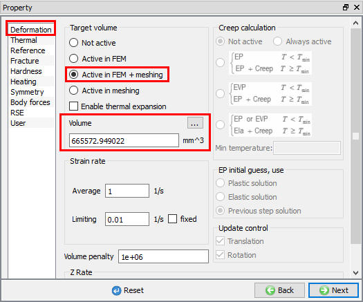
Workpiece Target volume

In the Property page, check Active in FEM + meshing , click to set Volume as the initial volume of the workpiece (see Fig. LAGEXL1.18.). Click on until to Control page.

Target volume setting of the workpiece

Controls

In the Control page. we can use to adjust the positions of objects.

All the die components were imported from the .stl files. The container and the die were in the correct locations. The ram is away from the workpiece. Since the workpiece was generated as a primitive within DEFORM, we need to move the ram down to touch the workpiece.

Click on and specify Interference positioning. Select the Ram as the Positioning object and the Workpiece as the Reference. Verify that the Approach direction is –Z. Click and then . Click on to Contact page.

Contact

In the Contact page, click on to create all the relationships of the workpiece with other objects. Then, let’s edit the parameters setting for contact relationships of the workpiece.

• Select the Ram – Workpiece relationship and click . Define contact separation as ‘Separable ‘, Shear friction as ‘1.0 ‘ and heat transfer coefficient as ‘11.0 ‘.

• Select the Container – Workpiece relationship and click . Define contact separation as ‘Separable ‘, Shear friction as ‘1.0 ‘ and heat transfer coefficient as ‘11.0 ‘.

• Select the Die – Workpiece relationship and click . Define contact separation as ‘Separable ‘, Shear friction as’ 0.4 ‘ and heat transfer coefficient as ‘11.0 ‘.

Click the to determine an intelligent contact tolerance. Click on to generate contact for all the relationships.

The contacts of the workpiece with other objects is shown in Fig. LAGEXL1.19. We can see contacts of the workpiece with the ram and the die. Currently there is no contact of the workpiece with the container because there is a gap between the two objects. The workpiece will expand to contact the container during the simulation. Click until to Step Control page.

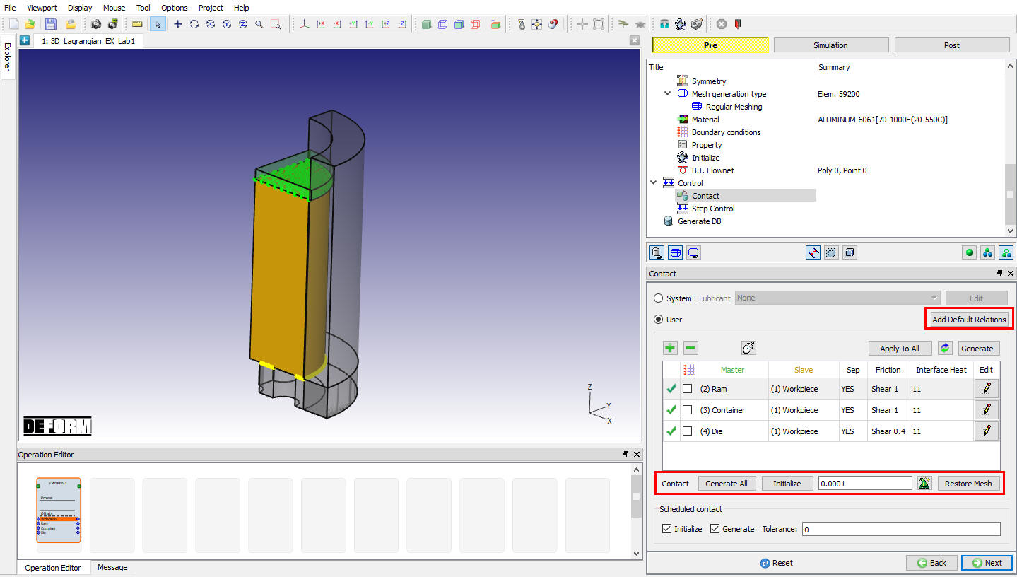
Contacts of the Workpiece

Step Controls

Click to switch to expert mode in the top menu bar for step control.

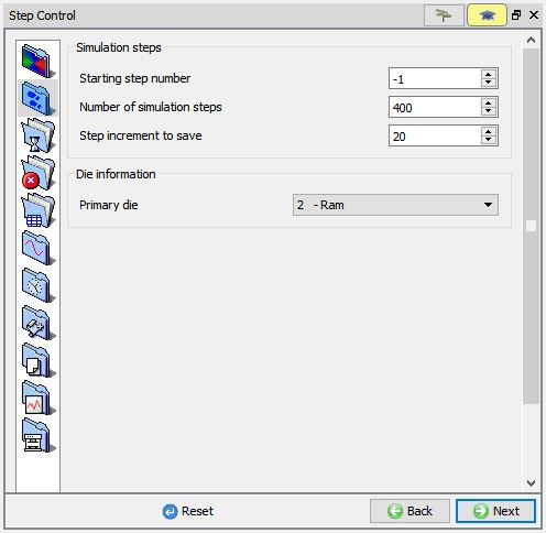
Simulation steps

InSimulation step dialog, set Number of simulation steps as 400 and Step increment to save as 20. Set Primary Die as ‘ 2 -Ram ‘ (see Fig. LAGEXL1.20.).

Simulation step setup

Step increment

In Lagrangian extrusion simulation, if there is a gap between the billet and the container, the first deformation stage is compressing the billet to fill the gap, the second deformation stage is extruding process.

For extrusion simulation, the general rule to set up step increment is that we do not want the material to flow more than 1/3 of their element size in any step.

In order to set up step increment correctly, we should learn about some basic extrusion parameters of the application.

In this example, for the quarter model, the entry area is 3846.50 mm2, the exit area is 726.52 mm2. So, the extrusion ratio is 5.29.

If we use a billet with diameter of 138 mm and height with 178 mm in Lagrangian simulation, for the quarter model, the billet area is 3737.39 mm2. The volume gap between the billet and the container is 19421.58 mm3 ((3846.50-3737.39)*178). The height for the billet to fill the volume gap is 5.20 mm (19421.58/3737.39). If the movement velocity of the ram is 4 mm/s, then the time to fill the volume gap is 1.30 s.

Based on above understanding, we can set different step increments in different deformation stages. In the gap filling stage, the minimum element size is 2 mm, the movement velocity of the ram is 4 mm/s, so the appropriate time/step of the ram would be 0.17 sec/step. In the extruding stage, the minimum element size is 2 mm, the movement velocity of the extrudate is 21.16 mm/s, so the appropriate time/step of the ram would be 0.03 sec/step.

In the Step increment dialog, set Solution step definition as Time. Set Step increment control to f(stroke) and click . Set the function as shown in Fig. LAGEXL1.21. and then click and .

Stroke	Step definition
0	0.17
5.2	0.17
5.21	0.03
200	0.03

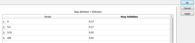
Step definition

By the way, if the gap is very small, we can also use a constant step increment with the appropriate time/step of the extruding stage for the whole deformation process.

Stop criteria

In the Stopping criteria dialog, define Primarydiedisplacement Z as 28 mm as show in Fig. LAGEXL1.22.

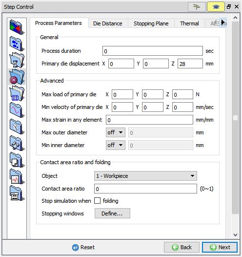
Stopping control

Double constraints settings

In order to ensure that no velocity leaks occur in the die and allow the correct outlet velocity to be calculated, it’s better to set double constraints on edges for extrusion.

In the Control files dialog, check Double constraints on edges , set Anglerangefrom75 deg to 105 deg, also check Include convex edges (see Fig. LAGEXL1.23.). Click on to Generate DB.

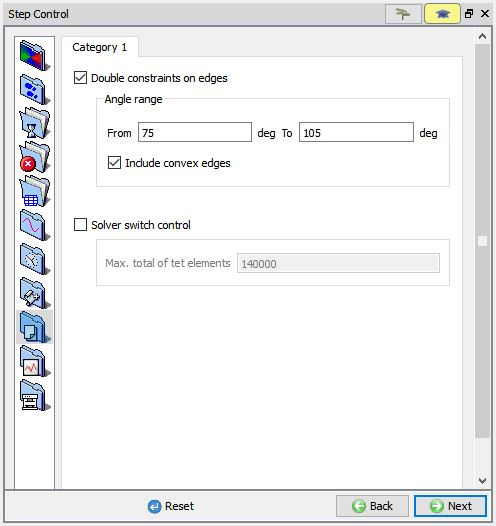
Double constraints setting

Generate DB

Click to see if anything was missed in the setup and then click on the button to generate the database. Observe the message in Message tab informing database generation status.

Running Simulation

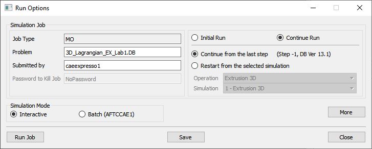
Once the database has been generated switch to the Simulation mode by clicking on button above the operation tree. Click on the action label to open the Run Options dialog as shown in Fig. LAGEXL1.24. Use the default ContinueRun option to select “Continue from the last step ” (from step -1) option and then select the Simulation mode as Interactive radio button. Click on button to run the simulation.

To define MPI settings, click on button, Run Options window will expand and displays options to define MPI settings for simulation (max number of processors that can be defined depend on your 3D MPI license).

Run Simulation Window

Monitor the progress of the simulation by looking at the Simulation Message and Simulation Log tab, make sure that the option is checked. User can view the Extrusion process from simulation graphics as the simulation proceeds to the specified Step definition.

Post Processing

From the message file, we can see that ‘PROGRAM STOPPED!’ and ‘THE Z STROKE 28.0000000 HAS REACHED THE SPECIFIED LIMIT 28.0000000’ after step 215.

When the simulation is completed, review the results by switching to Post mode using the button above the Simulation tool bar.

Play through the steps of the simulation and look how the workpiece flows in extrudate region in Lagrangian extrusion operation. From the simulation results, we can see that surround profiles (D2 & D3) are bending toward the central profile (D1) during the extrusion process.

Plots of the Effective strain and Temperature of the workpiece at last step are given in Fig. LAGEXL1.25. and Fig. LAGEXL1.26.

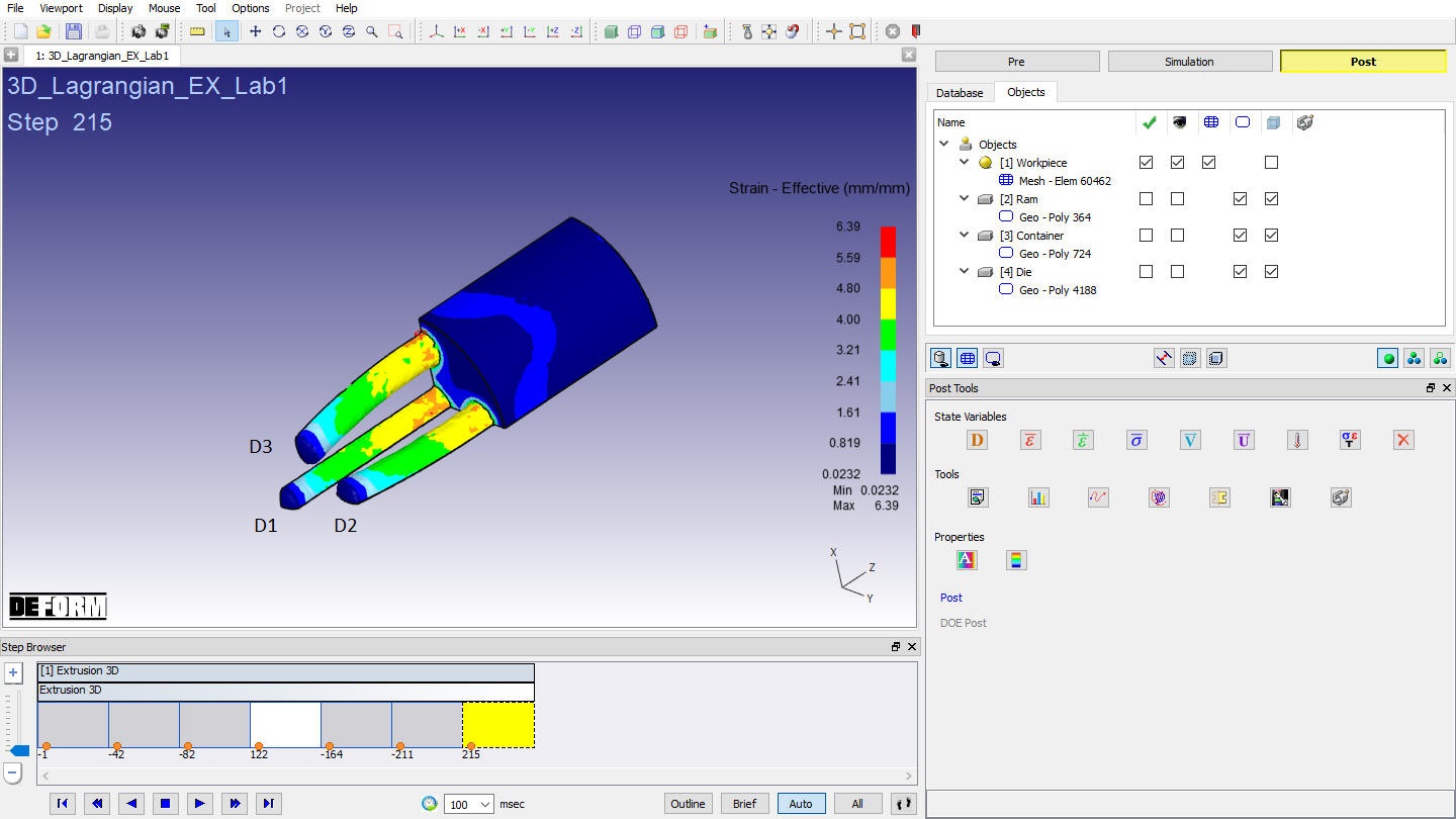
Effective strain distribution of the workpiece at last step

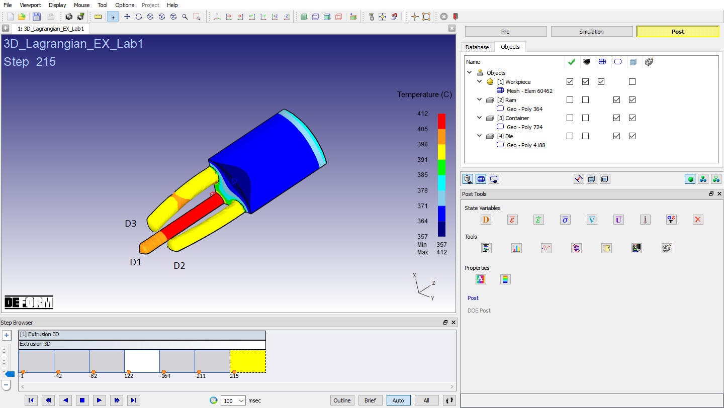
Temperature distribution of the workpiece at last step