3D HEAT TREATMENT BATCH FURNACE TEMPLATE LAB
Problem Summary
The Heat Treatment Batch Furnace template in new MO (Multiple Operations) is a convenient tool to set up a multiple-operation process for modeling loads of multiple workpieces and fixtures heating in the batch furnace, following a prescribed time and temperature setting points (thermal schedule).
This lab will demonstrate how to use this template to prepare a furnace heating simulation of a round load of 6 steel parts. This lab can also help users understand the capabilities of new MO.
Starting a Multiple Operations problem
Create a new problem either by selecting File ![]() New Problem or by clicking the New Problem
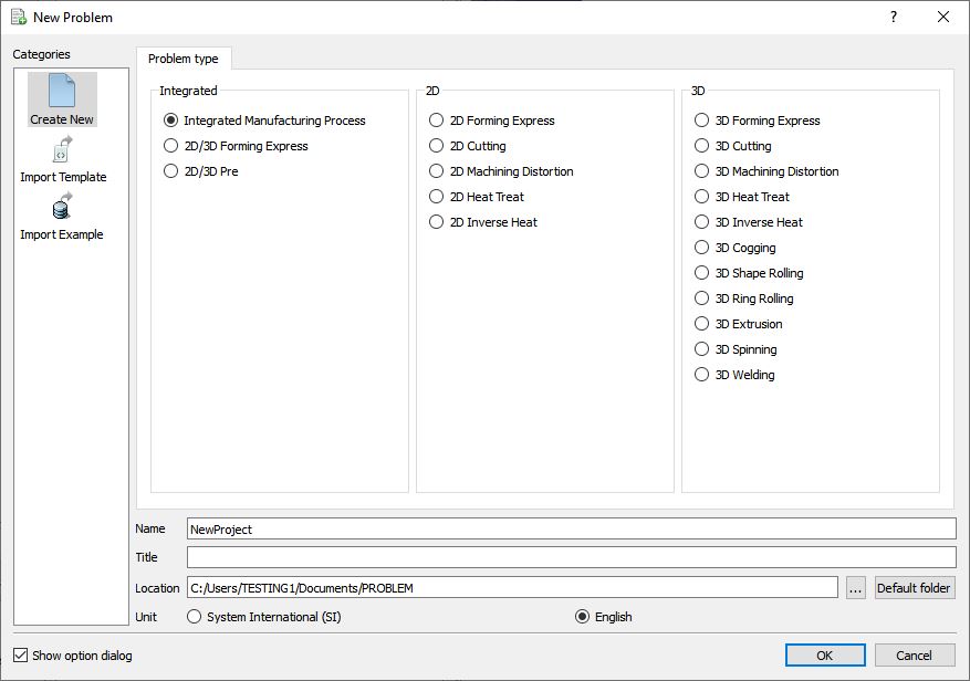
New Problem or by clicking the New Problem ![]() icon. The Problem Setup window will appear. Select “Integrated Manufacturing Process “ radio button and unit system as “English “ radio button in unit field as shown in Fig. 3FHL1.1. Define Problem Name as “**DrillBit** “ and make sure the “Show option dialog” check box is turned on (if we do not turn on the “Show option dialog ” check box, then we will not get the New Project dialog in MO UI). Then click on
icon. The Problem Setup window will appear. Select “Integrated Manufacturing Process “ radio button and unit system as “English “ radio button in unit field as shown in Fig. 3FHL1.1. Define Problem Name as “**DrillBit** “ and make sure the “Show option dialog” check box is turned on (if we do not turn on the “Show option dialog ” check box, then we will not get the New Project dialog in MO UI). Then click on ![]() button to open a new Problem using the Deform Integrated Manufacturing Process.
button to open a new Problem using the Deform Integrated Manufacturing Process.
Problem type selection window
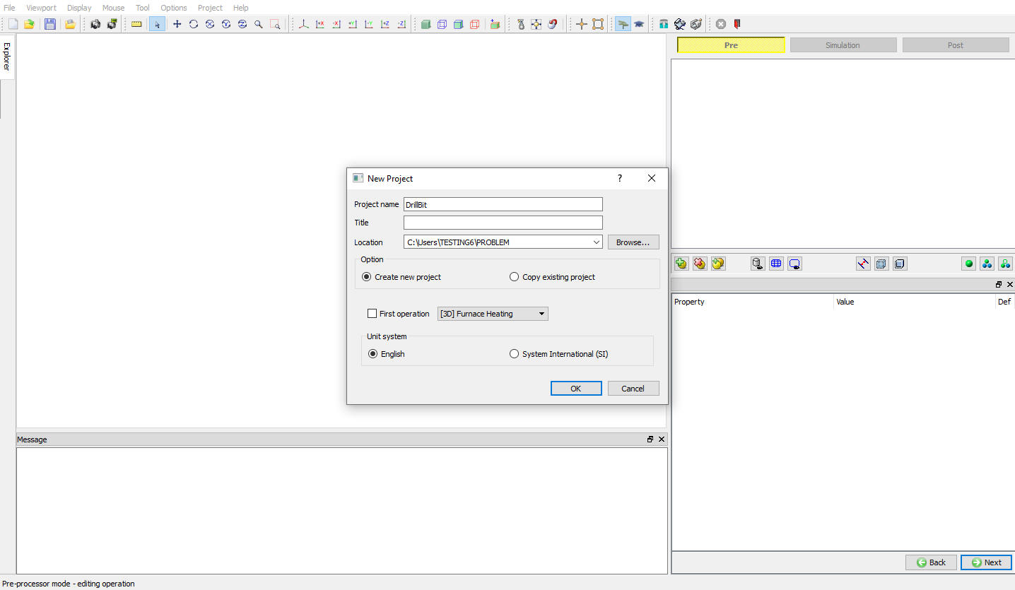
Multiple operation wizard will open with the New Project dialog (see Fig. 3FHL1.2.), at this point user will be prompted to specify a project name (system will create a separate folder with this project name) and title for this session. In this session we use ‘DrillBit ’ as the project name, English unit system and click on ![]() button to create the project.
button to create the project.
DEFORM New Multiple operation Main window
At ‘Location’ the new project ant its folder will be created as shown in see Fig. 3FHL1.3.
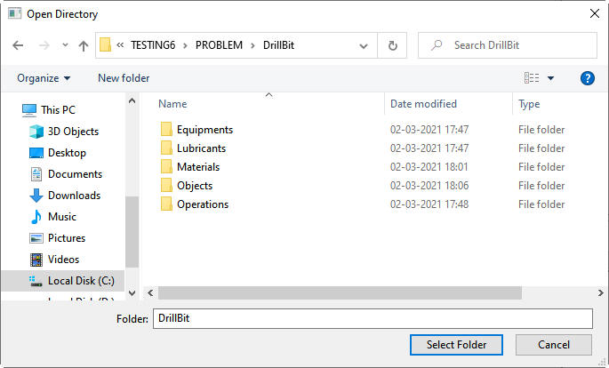
New Project ‘DrillBit’ folder
Add a Heat Treatment Batch Furnace Module to Project
To add a ‘Furnace Heating’ process to MO. Move the mouse to the MO main window on the left, hang on the ‘Explorer’ tag. There will be a ‘Explorer’ window expanded from left to right, see Fig. 3FHL1.4.
Adding Furnace Heating process to the MO project
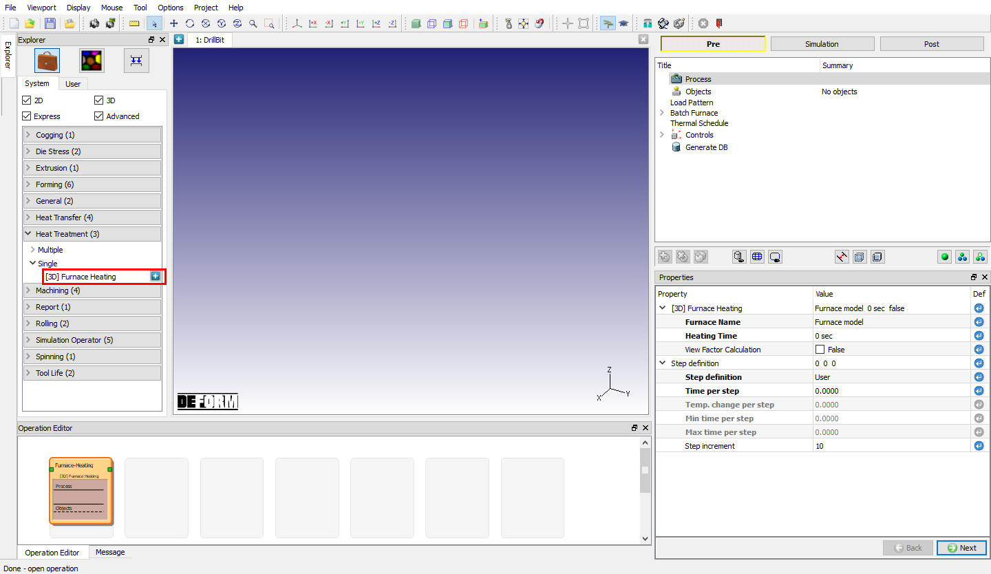
On ‘Explorer’ window, click on ‘Heat Treatment (3) ‘, then ‘Single ‘ and under ‘Single ‘ category, Click on the ![]() (Add) icon right to ‘[3D] Furnace Heating ‘ as shown in Fig. 3FHL1.4. as this lab will demonstrate how to use the new MO to prepare a furnace heating simulation of multiple steel parts with specific load pattern. This will add a 3 dimensional heat treatment furnace heating process to the project, as evidence, an graph item was inserted in the ‘Operation Editor’, which can be seen at Fig. 3FHL1.5. Click on the item
(Add) icon right to ‘[3D] Furnace Heating ‘ as shown in Fig. 3FHL1.4. as this lab will demonstrate how to use the new MO to prepare a furnace heating simulation of multiple steel parts with specific load pattern. This will add a 3 dimensional heat treatment furnace heating process to the project, as evidence, an graph item was inserted in the ‘Operation Editor’, which can be seen at Fig. 3FHL1.5. Click on the item  , the tree structure, which is the ‘Navigator’ window on the right side of the MO main window will be rebuilt based on the predefined template type, see Fig. 3FHL1.5.
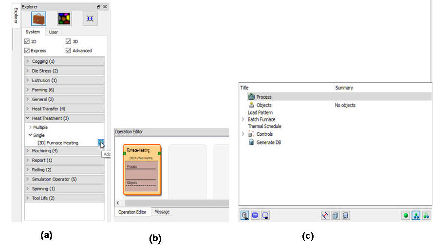
MO Windows; (a) Explorer window (b) Operation Editor Window (c) Operation tree window
The tree structure in the ‘Operation tree’ window shows the items which will need to be configured for the ‘Furnace Heating’ simulation. Click on any item go to the corresponding configuration window, or click on ![]() and
and ![]() button on the bottom right going back and forth between different configuration windows.
button on the bottom right going back and forth between different configuration windows.
In the following chapters, we will go through each configuration window.
Configure Process
‘Process’ window is mainly list a few parameters (Properties), it’s a summary of the project information as shown in Fig. 3FHL1.6. Also some controls can be modified quickly without going through the individual configuration windows.
Process page
Click on ![]() to select the objects.
to select the objects.
Define Workpiece
In this lab only Workpiece is used, so keep 1 workpiece radio button selected (see Fig. 3FHL1.7.) and click on ![]() to define workpiece.
to define workpiece.
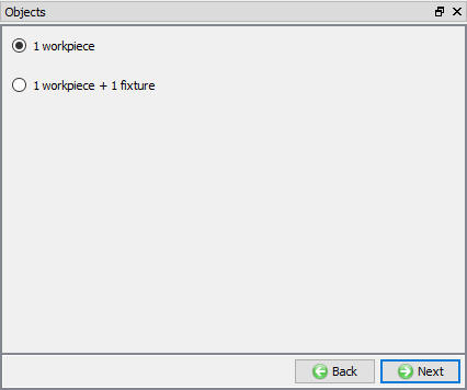
Objects selection window
Name the Object
Type in ‘Drill Bit ‘ as object name, leave all others as default as shown in Fig. 3FHL1.8. Then click on ![]() to the ‘Geometry’ definition page as shown in Fig. 3FHL1.9.
to the ‘Geometry’ definition page as shown in Fig. 3FHL1.9.
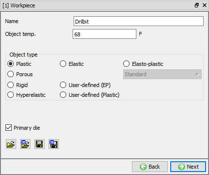
Workpiece object definition window
Workpiece geometry definition window
Create Geometry
On ‘Geometry’ page, click on ![]() , on the following window choose ‘Cylinder ‘ and give 9.8 inch as diameter and 24 inch as height as shown in Fig. 3FHL1.10., the object geometry is also previewed at the central graphic window area. Click on
, on the following window choose ‘Cylinder ‘ and give 9.8 inch as diameter and 24 inch as height as shown in Fig. 3FHL1.10., the object geometry is also previewed at the central graphic window area. Click on ![]() button to accept all the changes, and it will come back to the ‘Geometry’ definition, click on
button to accept all the changes, and it will come back to the ‘Geometry’ definition, click on ![]() to the ‘Mesh’ page, see Fig. 3FHL1.11.
to the ‘Mesh’ page, see Fig. 3FHL1.11.
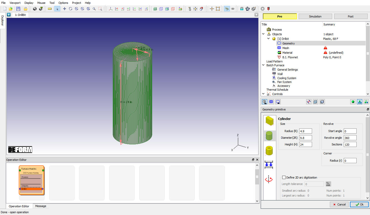
Geometry primitive settings to create the ‘Drill bit’ part
Mesh the Object
Only ‘Tetrahedral Mesh’ can be generated in this template, put 5000 in ‘Target number of Elements’ and then click on ![]() . The mouse icon on the screen turns to busy and then back to normal, which indicating the mesh has been generated, the results are also plotted on the central graphic area, see Fig. 3FHL1.11. User can preview the mesh by clicking on
. The mouse icon on the screen turns to busy and then back to normal, which indicating the mesh has been generated, the results are also plotted on the central graphic area, see Fig. 3FHL1.11. User can preview the mesh by clicking on ![]() , as this only generate the surface mesh it will be quick. Click on
, as this only generate the surface mesh it will be quick. Click on ![]() , go to the ‘Material’ page, see Fig. 3FHL1.12.
, go to the ‘Material’ page, see Fig. 3FHL1.12.
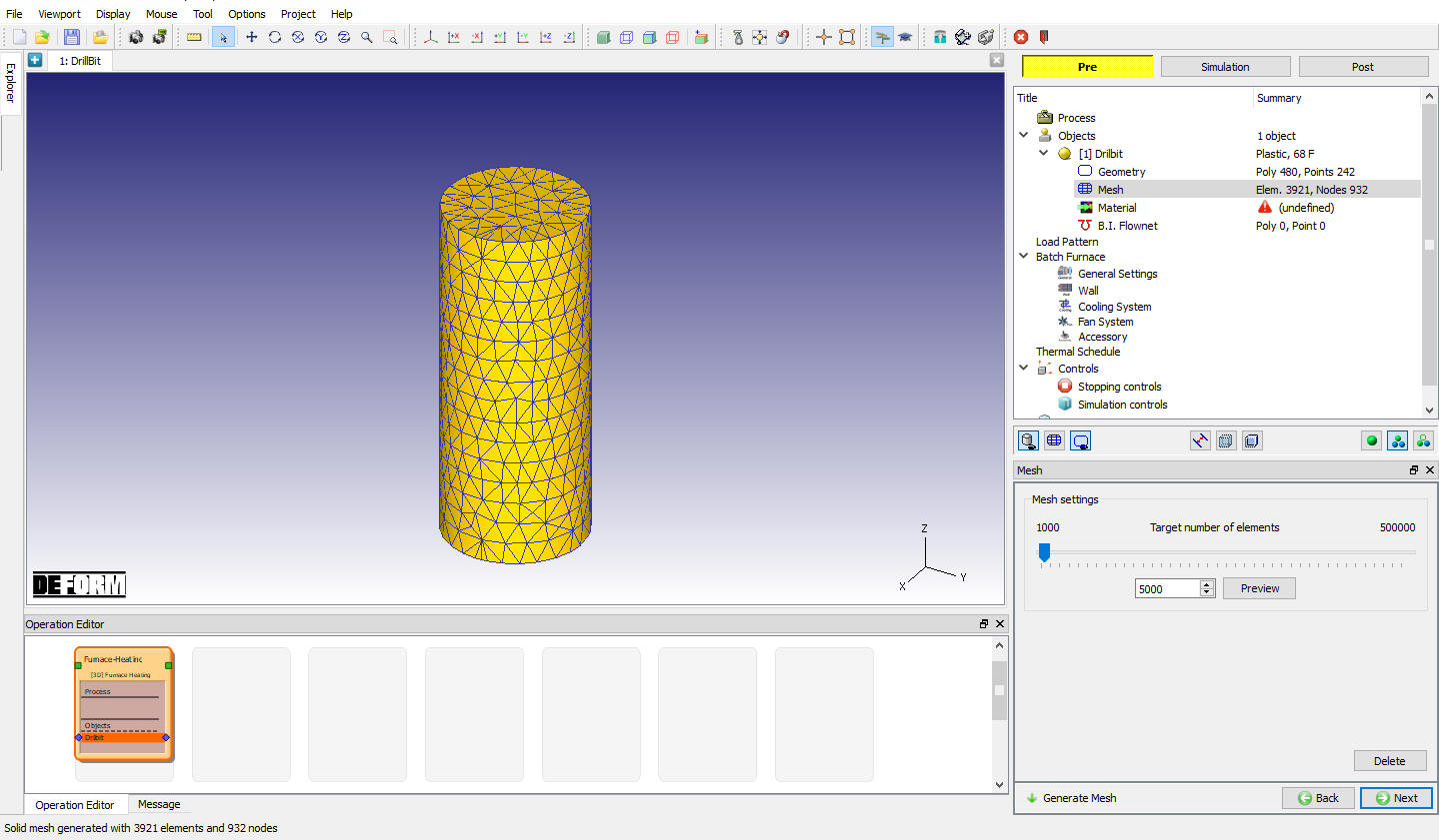
Mesh generation
Load and Assign Material
On the object ‘Material’ selection window, click on ![]() (Load material from a file) “4340.key “ from \3d\LABS\Furnace_Material folder in installation path as shown in Fig. 3FHL1.12. System automatically assign the loaded material for workpiece. Click on
(Load material from a file) “4340.key “ from \3d\LABS\Furnace_Material folder in installation path as shown in Fig. 3FHL1.12. System automatically assign the loaded material for workpiece. Click on ![]() to define the Load pattern window.
to define the Load pattern window.
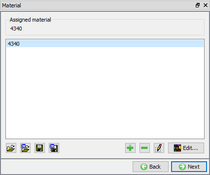
Load and assign material from library
Define Load pattern
Modeling a load of multiple parts heated up in the batch furnace, to define load pattern. A round pattern with 6 parts will be created, so choose ‘Round’ Pattern type, type in 6 in the ‘Row’ column, the distance between workpieces is 17 inch and leave the ‘Central symmetry’ checked, see Fig. 3FHL1.13. Finish the load pattern definition, the pattern can be previewed by clicking on the button, the result is plotted in the central graphic window area, see Fig. 3FHL1.13.
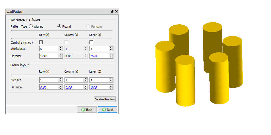
Load Pattern design of parts; Load pattern definition window and Preview of load pattern
Batch Furnace Definition
Furnace definition will be introduced in this section, click on the tree, the triangle button beside  to unfold ‘Batch Furnace ‘ definition item, under it, there will be several sub-items need to be configured.
-
 Basic furnace information, like shape, size and heat source etc.
 -
 Furnace wall information, include material, number of layers and thickness.
 -
 Cooling related parameters, for example, water rate of the cooling, inlet and outlet water temperature.
 -
 Recirculation fan settings, fan’s size, material and speed etc.
 -
 Accessory information, this is designed for the estimation of the heat absorbed by any small furnace parts, which no need to be meshed, assuming its temperature is uniform and same as that of the furnace.
Click on the tree the furnace definition item  will led to main ‘Batch Furnace’ window as shown in Fig. 3FHL1.14.
Batch Furnace main definition window
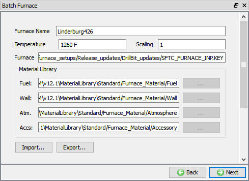
Set ‘Furnace Name’ as ‘Linderburg426 ‘, the initial ‘Furnace Temperature’ as 1260 F. Then click on ![]() to accept it and go to ‘General Settings’ window ().
to accept it and go to ‘General Settings’ window ().
*Note that ‘Scaling’ is the scaling factor of the model, it’s not recommended since it require the special boundary condition set up, leave it as 1.
General settings
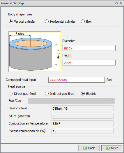
The Linderburg426 batch furnace’s Body shape is ‘Vertical Cylinder ‘, the overall size are 99.6 inch as diameter and 72 inch high. It’s electric furnace, the Connected Heat Input is 113.727 Btu/sec.
Finish all the settings, see Fig. 3FHL1.15., then click on ![]() to accept it and go to ‘Wall’ definition window ().
to accept it and go to ‘Wall’ definition window ().
General Settings
Wall
On the ‘Wall’ definition page, there will be three group of information need to be input, ‘Roof’, ‘Side wall’ and ‘Bottom’.
Load and assigning material for wall
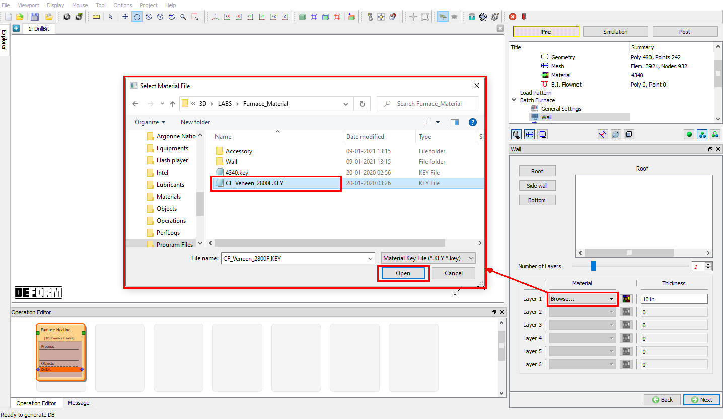
The default is the ‘Roof’ information, set number of layers as 1 , thickness as 10 inch, see Fig. 3FHL1.16.
To assign layer’s material, click on the ‘Material ‘ pull down list by ‘Layer 1 ‘, as seen in Fig. 3FHL1.17. move the mouse to ‘Browse… ‘ and select the “CF_Veneen_2800F.key “ material keyword file from \3d\LAB\Furnace_Material folder in installation path. As results,’CF_Veneen_2800F’ is added to this pull down list and chosen as the current material for layer 1. Furthermore it’s also available for ‘Side wall’ and ‘Bottom’. Meanwhile, ‘Drag and Drop’ material method is also supported, by doing so, drag the material name from ‘Material’ explorer ( Fig. 3FHL1.17.) and drop it on the material pull down list.
Notice the![]() beside the material name
beside the material name  , click on this button will let to the ‘Material Editor’ page (Fig. 3FHL1. Fig. 3FHL1.17.). Changes can be made on the current assigned material.
Then click on ![]() button, set number of layers as 1 , thickness as 9 inch, see Fig. 3FHL1.17.. From the material pull down list, choose,’CF_Veneen_2800F ‘ and assign it to layer 1 of side wall.
button, set number of layers as 1 , thickness as 9 inch, see Fig. 3FHL1.17.. From the material pull down list, choose,’CF_Veneen_2800F ‘ and assign it to layer 1 of side wall.
Then click on ![]() , set number of layers as 1, thickness as 9 inch, see Fig. 3FHL1.17. From the material pull down list, choose ‘CF_Veneen_2800F ‘and assign it to layer 1 of bottom wall.
, set number of layers as 1, thickness as 9 inch, see Fig. 3FHL1.17. From the material pull down list, choose ‘CF_Veneen_2800F ‘and assign it to layer 1 of bottom wall.
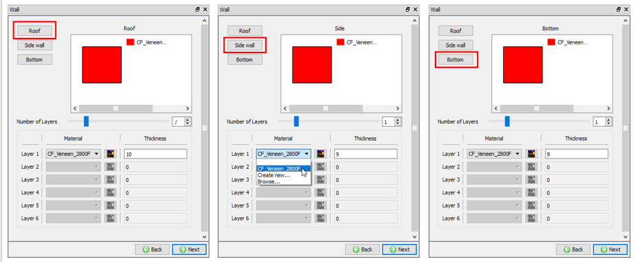
Wall Definition
Finish all the settings, then click on ![]() to accept it and go to ‘Cooling System’ definition window ().
to accept it and go to ‘Cooling System’ definition window ().
Cooling System
Leave all fields as zero for this lab, see Fig. 3FHL1.18. Click on ![]() , go to ‘Fan System’ definition window ().
, go to ‘Fan System’ definition window ().
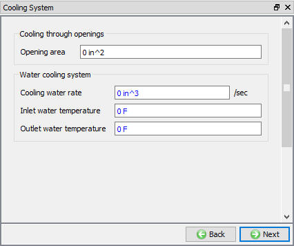
Cooling System Definition
Fan System
This is a vacuum furnace, so check ‘Non – atmosphere’  as shown in Fig. 3FHL1.19.
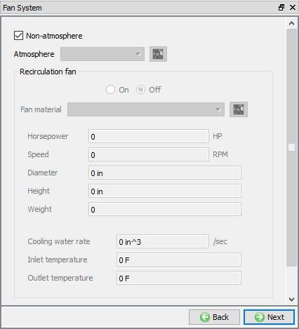
Fan system definition
Click on ![]() then go to ‘Accessory’ definition ().
then go to ‘Accessory’ definition ().
Accessory
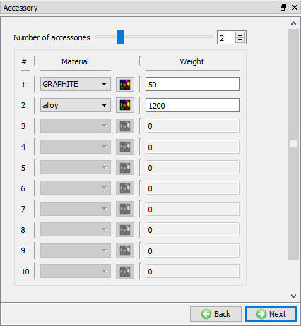
The total weight of heating elements of the Linderburg426 is 50 lbs, the material is graphite. Other than this, a total 1200 lbs of supports of alloy will also need to be considered in the heat estimation.
On ‘Accessory’ page, set number of accessories as 2, see Fig. 3FHL1.20., then assign material to the corresponding furnace parts.
Set accessory 1 as heating elements, in this lab, since the material keyword file for graphite is already prepared, just browse  from \3d\LABS\Furnace_Material\Wall\GRAPHITE.KEY in installation path to the ‘Accessory’ window on
  .
.
Then set accessory 2 as supports, similarly browse from \3d\LABS\Furnace_Material\Accessory\Alloy.KEY in installation path to the ‘Accessory’ window on  .
.
Set accessory 1 as heating elements, in this lab, since the material keyword file for graphite is already prepared, just browse  from \3d\LABS\Furnace_Material\Wall\GRAPHITE.KEY in installation path to the ‘Accessory’ window on .
Then set accessory 2 as supports, similarly browse from \3d\LABS\Furnace_Material\Accessory\alloy.KEY in installation path to the ‘Accessory’ window on.
Assign material to Accessory
Click on ![]() to accept changes. Up to here, the furnace definition has been done, furnace Linderburg426 has been successfully created and configured.
to accept changes. Up to here, the furnace definition has been done, furnace Linderburg426 has been successfully created and configured.
*Note that on ‘Batch Furnace’ main definition page ( Fig. 3FHL1.15 ), there are four furnace material related settings,

- gas/fuel material sub folder

- layer material of the furnace wall

- furnace atmosphere

- accessory material
These settings are the default material sub folder where to locate corresponding material keyword files, so any material keyword file presented in these folders will be list out in the corresponding material comb box, as seen in Fig. 3FHL1.15.
Thermal Schedule and PID Control
Thermal Schedule
Thermal schedule are the time and temperature setting points, to define it, click on the tree the ‘Thermal Schedule’ item  .
.
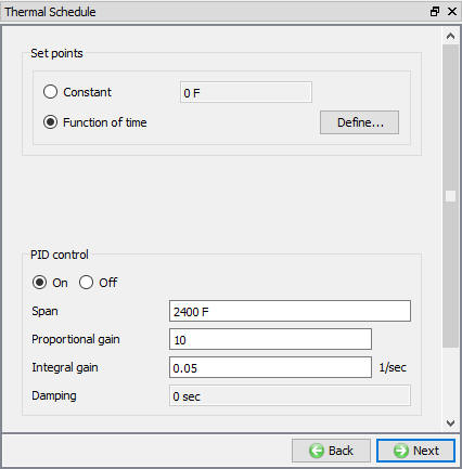
On the following ‘Thermal Schedule’ definition window, as seen on Fig. 3FHL1.21., select  and then click on
 ![]() button.
button.
Thermal Schedule definition
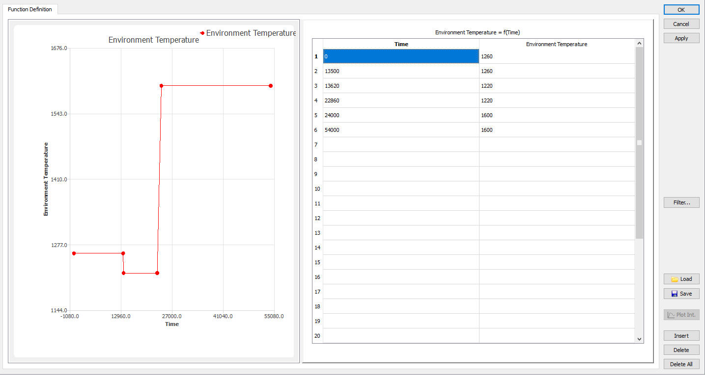
Then on the central window area, the ‘Environment Temperature’ function definition window will show up, on the table, input the following ‘time (s)/temperature (F)’ data pairs ‘0/1260’, ‘13500/1260’, ‘13620/1220’, ‘22860/1220’, 24000/1600’, and ‘54000/1600’. Click ![]() to review the function as curve plotting as shown in Fig. 3FHL1.22.
to review the function as curve plotting as shown in Fig. 3FHL1.22.
Environmental function definition
Click on ![]() to accept the values.
to accept the values.
PID Control
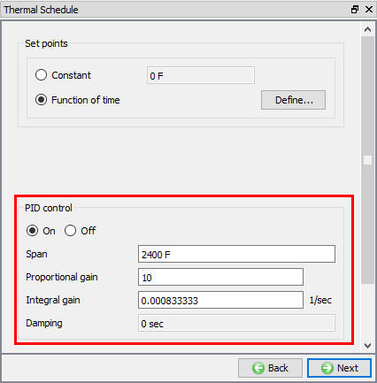
Back to the ‘Thermal Schedule’ definition page as seen in Fig. 3FHL1.23.
Turn on PID control by click on  . Then set ‘Spain’ to 2400 F, ‘Proportional Gain’ to 10 , ‘Integral Gain’ to 0.000833333 1/sec and leave ‘Damping’ as zero.
PID Control definition
Next click on ![]() to accept PID settings and click on
to accept PID settings and click on ![]() for positioning and stopping controls window as there is no positioning is required and process duration stopping controls will be defined in the simulation controls heating time as shown in Fig. 3FHL1.24 .
for positioning and stopping controls window as there is no positioning is required and process duration stopping controls will be defined in the simulation controls heating time as shown in Fig. 3FHL1.24 .
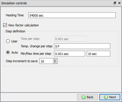
Simulation Control
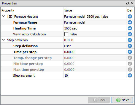
Check Viewfactor calculation check box to turn on Radiation, enter the Heatingtime as 54000 seconds and select Auto step definition radio button to define temperature based step definition. Leave the default Step definition values that is, Temperature change per step 5F, Min/Max time per step 0.001 and 10 seconds respectively.
Simulation Control
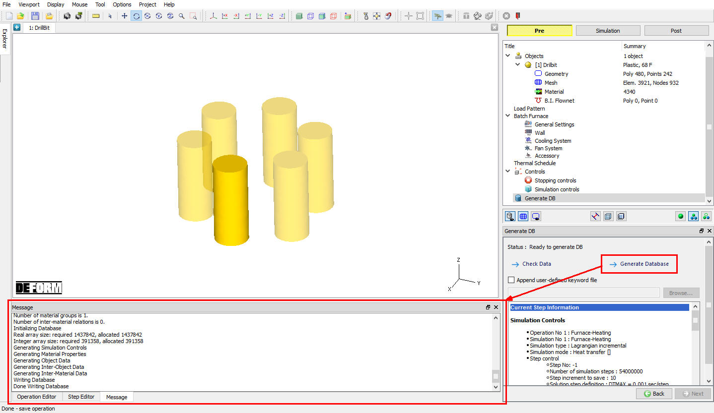
Generate Database
On ‘Generate DB’ page, click on ![]() , as seen in Fig. 3FHL1.25., the ‘Message’ window area, Database has been successfully generated.
, as seen in Fig. 3FHL1.25., the ‘Message’ window area, Database has been successfully generated.
Generate Database window
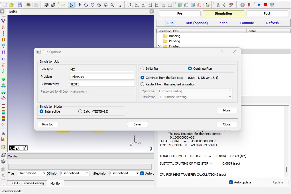
Run Simulation
Click on the ![]() action label to open the Run Options dialog as shown in Fig. 3FHL1.26. Use the default Continue Run option to select “Continue from the last step ” option and then select the Simulation mode as Interactive and click on
action label to open the Run Options dialog as shown in Fig. 3FHL1.26. Use the default Continue Run option to select “Continue from the last step ” option and then select the Simulation mode as Interactive and click on ![]() button to run the simulation.
button to run the simulation.
Run Simulation
*Note: Please make sure only use one processor, the furnace model does not support multiple cores yet.
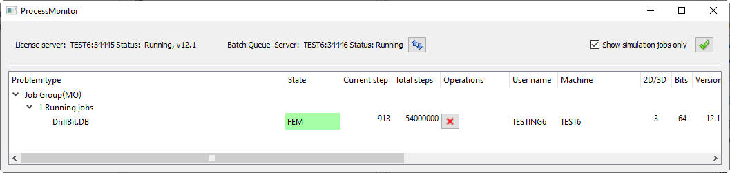
Click on the menu ‘Simulation’ ‘Process Monitor’, ‘Process Monitor’ window will be popped up as seen in Fig. 3FHL1.27., the running database ‘DrillBit’ information is list under ‘Running Jobs’.
Process Monitor
In the ‘Message’ window, it can be seen that the running job information are also updated frequently.
Post-Processing
Once the simulation is completed click on ![]() tab to post-processor the DB. The furnace energy consumption related information will be available other than the deform state variables like workpieces temperature.
tab to post-processor the DB. The furnace energy consumption related information will be available other than the deform state variables like workpieces temperature.
Energy Consumption
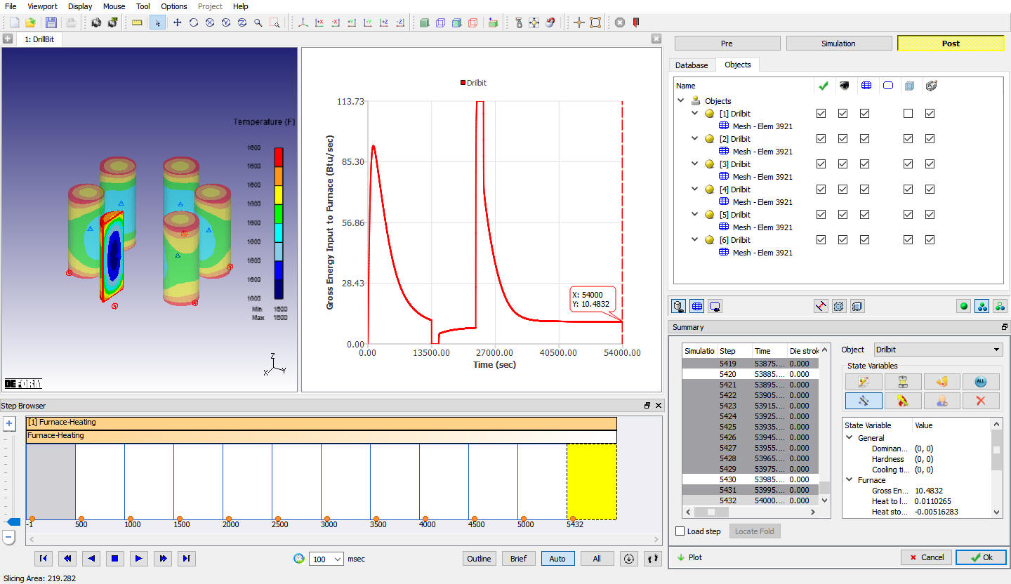
As seen in Fig. 3FHL1.28., in the post-processor, click on ![]() (Summary) button to view the simulation summary. On the ‘Summary’ window, click on Heat Treat then
(Summary) button to view the simulation summary. On the ‘Summary’ window, click on Heat Treat then  .
.
Furnace energy consumption curve
As showing in Fig. 3FHL1.28, on ‘Furnace’ summary page, there are several furnace related energy consumption variables,
-
Gross Energy Input - run time input energy value vs time.
-
Heat to load - run time heat absorbed by all the workpieces.
-
Heat stored in furnace - run time heat absorbed by all the furnace walls.
-
Water cooling - run time heat contents taken away by cooling water.
-
Loss through wall - run time radiation loss through the hot walls.
-
Loss through openings - run time radiation loss through any open areas like holes on the furnace wall.
-
Cool by fan - run time heat to the recirculation fan’s cooling water system.
-
Fan generated heat - run time heat generated by the recirculation fan as it’s ruining.
-
Furnace temperature – simulated furnace temperature.
-
Set point – thermal schedule.
Click on the ![]() button after selecting any variable, the corresponding energy consumption curve which is run time heat value vs time will be plotted on the graphic window area, as seen in Fig. 3FHL1.28.
button after selecting any variable, the corresponding energy consumption curve which is run time heat value vs time will be plotted on the graphic window area, as seen in Fig. 3FHL1.28.
Point tracking of temperature at different location
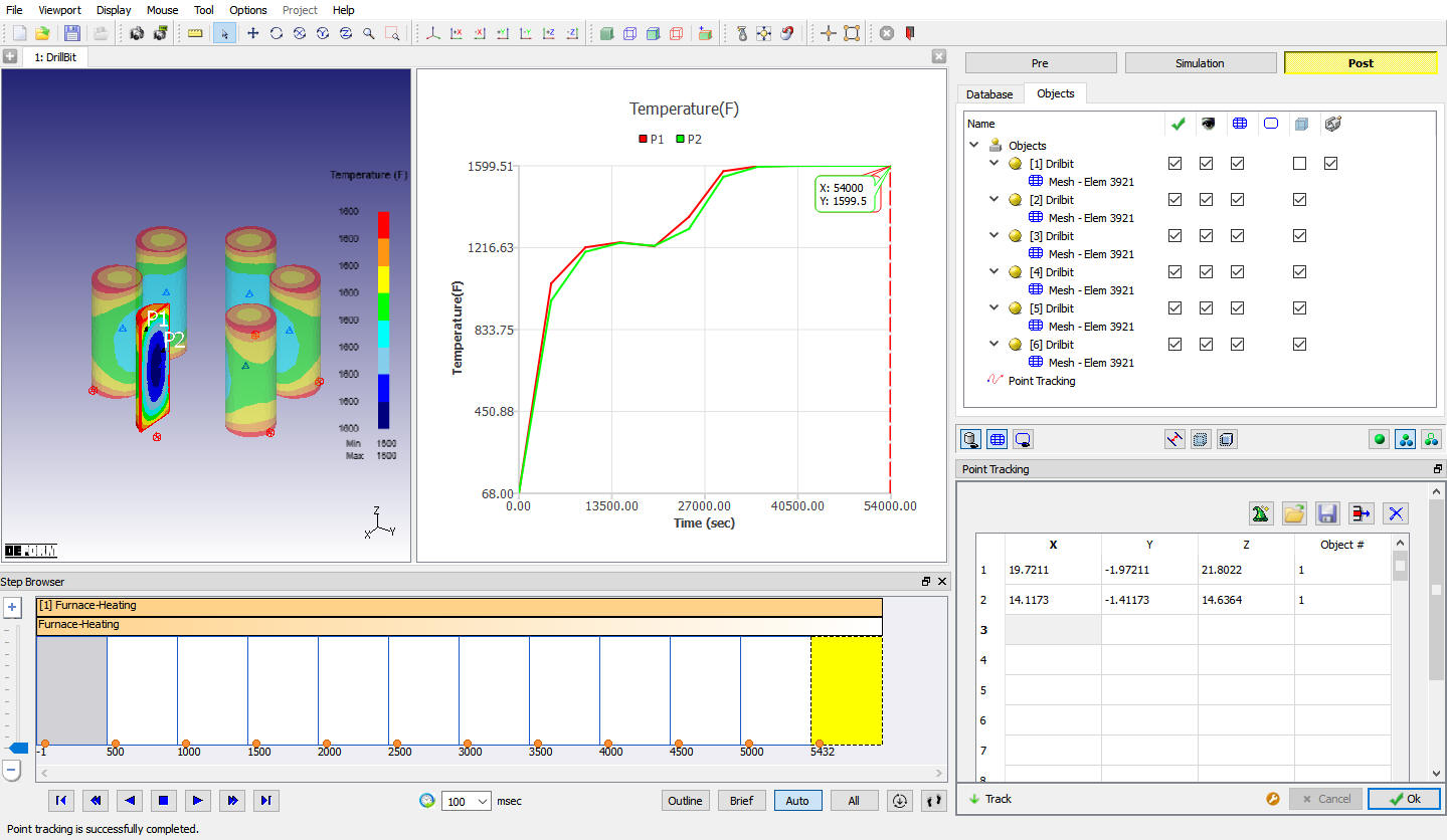
The point tracking is a very useful tool to check the temperature distribution among the load pattern.
As seen in Fig. 3FHL1.29, pick two points as corner and center respectively, select all steps, then point track the temperature, results are plotted in Fig. 3FHL1.29.
Point tracking points
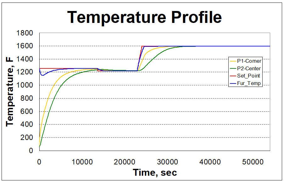
From Fig. 3FHL1.30, it shows that the corner and center of the workpiece are heated up almost at the same rate, so the temperature difference is relative smaller and this is very helpful to control the heat treatment quality. (Data are exported from the point tracking graph, and the summary graph of set point, furnace temperature)
Temperature profile
Related Topics:
6.2. Integrated Manufacturing Process Simulation layout