Lab1: Shot Peening Lab

This lab will demonstrate the setting up of shot peening of helical gear using Shot peening template.

1.1. Launching Shot Peen wizard

1.2. Creating New Project

1.3. Defining Shot Peening Process parameters

1.4. Loading material for helical gear

1.5. Defining Stress Input

1.5.1. Setting up Micro model (2D)

1.5.2. Run

1.5.3. 2D micro model impact stress and residual stress output

1.5.4. Measured Residual stress

1.6. Defining 3D model for shot peening

1.6.1. Defining Workpiece

1.6.1.1. Workpiece object page

1.6.1.2. Defining Workpiece geometry

1.6.1.3. Defining Material for Workpiece

1.6.1.4. Generating mesh for Workpiece

1.6.1.5. Assigning boundary conditions to Workpiece

1.6.1.6. Defining Workpiece movement

1.6.2. Defining Nozzle #1

1.6.2.1. Nozzle#1 Object definition

1.6.2.2. Defining Nozzle Location

1.6.2.3. Defining Nozzle movement

1.6.3. Positioning

1.7. Analysis of shot peening process

1.7.1. Particle Simulation

1.7.1.1. Particle Simulation settings

1.7.1.2. Particle Simulation Result

1.7.2. Impact simulation

1.7.2.1. Impact Simulation settings

1.7.2.2. Impact simulation result

1.7.3. Residual stress analysis

1.7.3.1. Residual stress analysis settings

1.7.3.2. Simulating Residual stress analysis

1.7.3.3. Residual Stress analysis results

Launching Shot Peen wizard

To launch Shot peening wizard, double click on “DEF_GUI_SHOTPEEN_64.EXE” in the installation directory of DEFORM software. Shot peening wizard looks like as shown in Fig. STPL1.1.

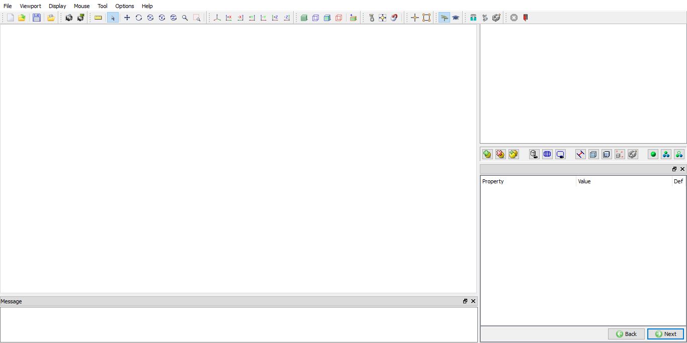
Shot peening wizard UI

Creating New Project

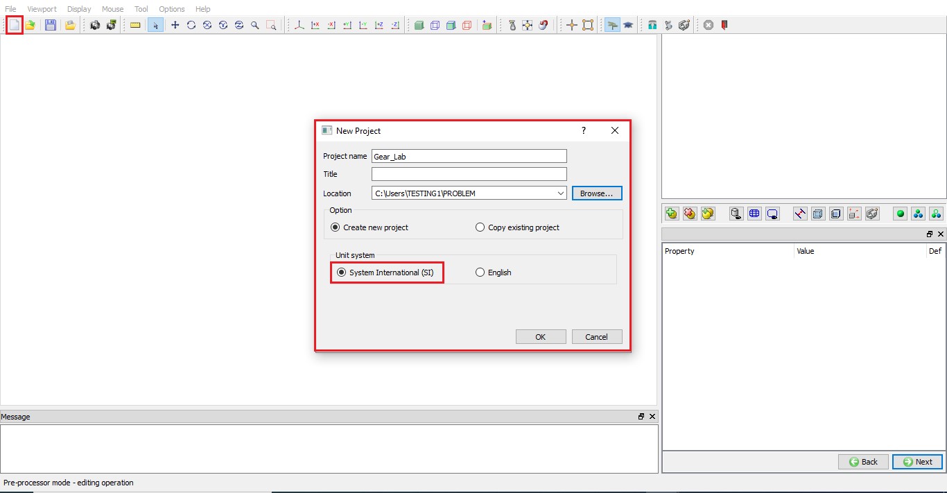
Create a new problem either by selecting File **New** or by clicking the New project icon. The New project window will appear (See Fig. STPL1.2.), define Project name as “Gear_Lab ” and select Unit system as “SystemInternational (SI) ” as shown in Fig. STPL1.2., click on button to open Shot peen project.

Creating New Project

A new tab Gear_Lab is added in UI and we can observe that shot peening operation tree is available to setup the process. “Shot Peen Process” window is opened by default to define shot peening process parameters, see Fig. STPL1.3.

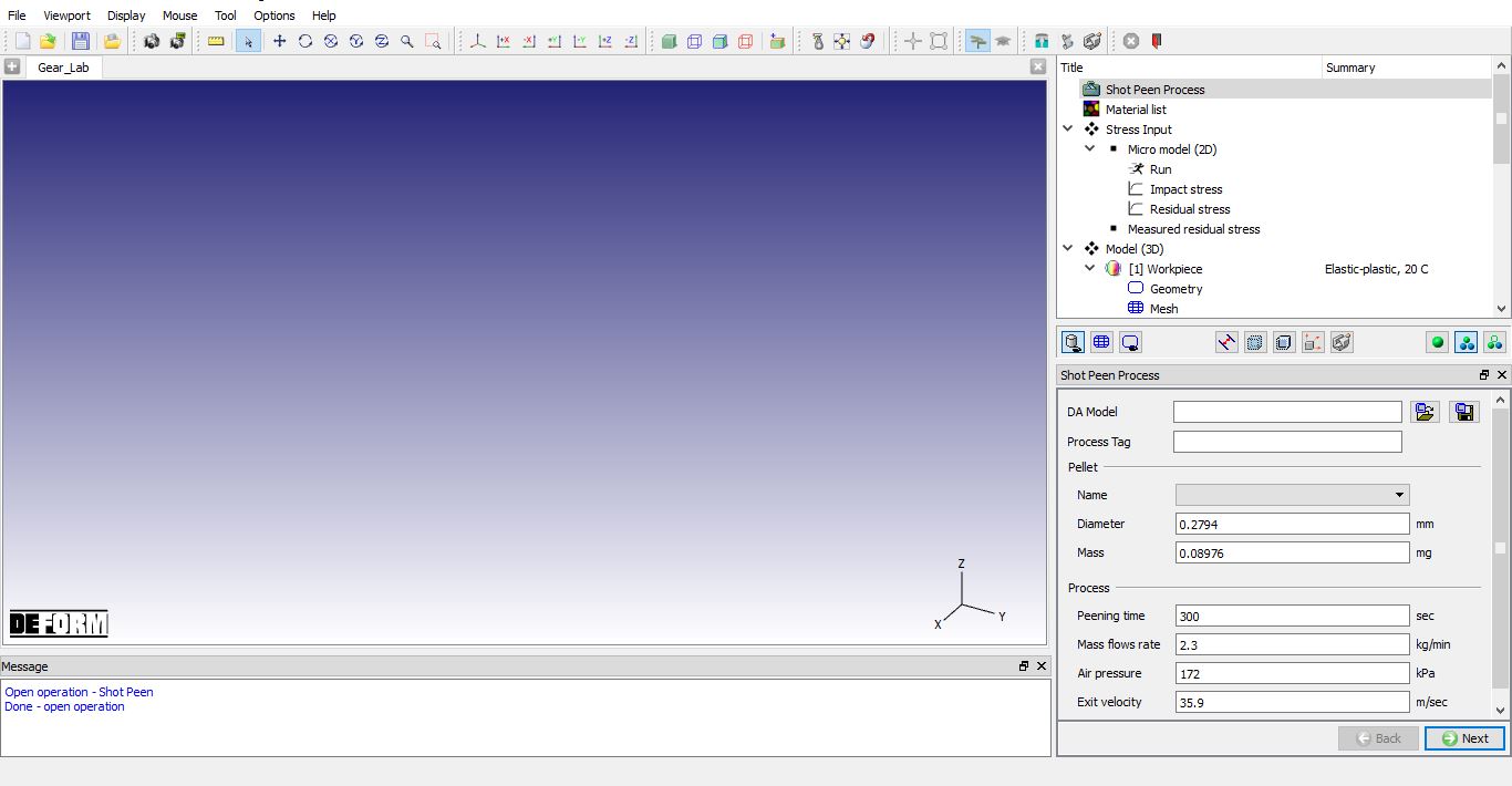
Shot Peening UI showing operation tree and Shot Peen Process window

Defining Shot Peening Process parameters

In Shot Peen Process page, we can import previously saved Data Analytics (DA) model file using button and by using option we can save the existing project DA model file to Library or inside the project folder.

In Process Tag field, we can enter Process information for Reference.

Under Pellet, Diameter of the pellet and its Mass can be defined. Select “New…” option using Name drop down field and define pellet Diameter as 0.2794mm and Mass as 0.08976 mg and save the DA model file inside the project folder using option. Also, we can load the saved pallet parameters by selecting respective name from Name drop-down list. Since we are simulating Shot peening operation for 20 seconds, define the Peening time as 20 sec as shown in Fig. STPL1.4. Under Process, we can define process parameters like Peening time, Mass flow rate, Air pressure and Exit velocity. Click on to Material list page.

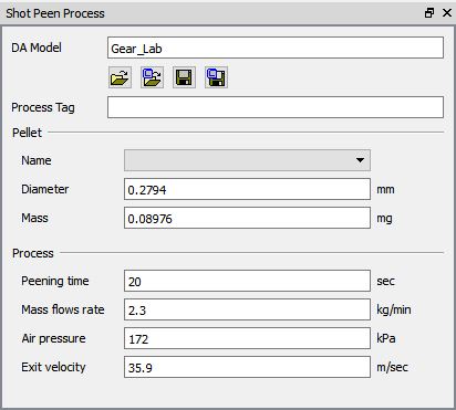
Defining shot peening process parameters

Loading material for helical gear

In material list page, click on (Load material from library) icon and load the material “AISI-302,COLD[70F(20C)] ” available under Stainless_steel group in material library as shown in Fig. STPL1.5.

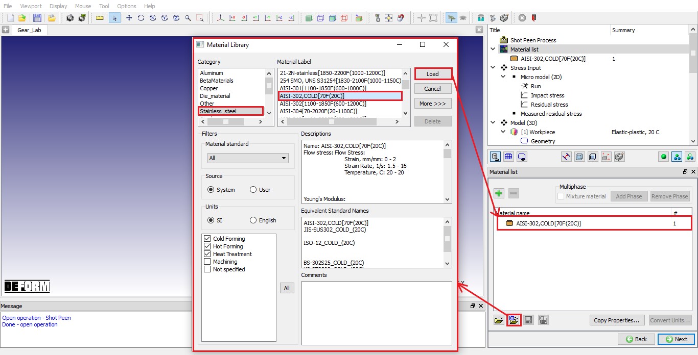
Loading material from library for helical gar

Defining Stress Input

The stress input values for object undergoing shot peening can be given either from simulated Micro model (2D) or from experimentally measured residual stress values. In this lab, we will use both Micro model (2D) and experimentally measured residual stress values.

Setting up Micro model (2D)

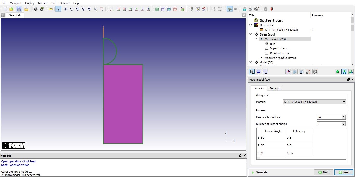
Click on “Micromodel (2D)” item in operation tree under stress input. under Process tab, by default material “AISI-302,COLD[70F(20C)]” is selected in list. Set Max number of hits as 10 and Number of impact angles as 3. Default Impact angles are 80, 50 and 20 with 0.5, 0.5 and 0.85 efficiency respectively as shown in Fig. STPL1.6.

Under Settings tab, we can define simulation control settings like time per step, number of steps and step increment to save for Loading simulation and Unloading simulation. In this lab, we will use default simulation control settings, so click on button to generate Databases for Micro model 2D simulation. An independent database each impact angle will be generated. Click on to Run page to simulate micro model 2D databases.

Process settings for 2D micro model simulation

Run

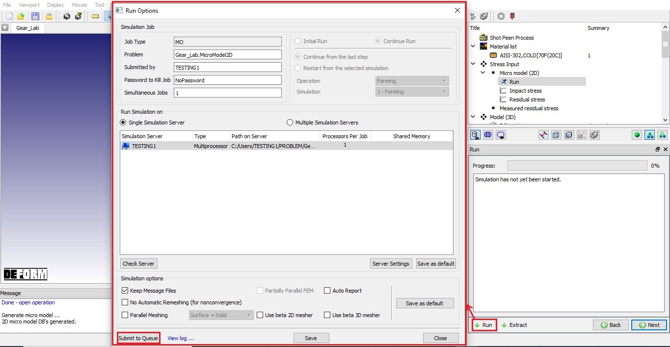
In Run page, we can simulate 2D micro model Databases using Run action button at the bottom (See Fig. STPL1.7.). When we click on , Run options dialog will be opened. Select simulation server and click on button to start the simulation.

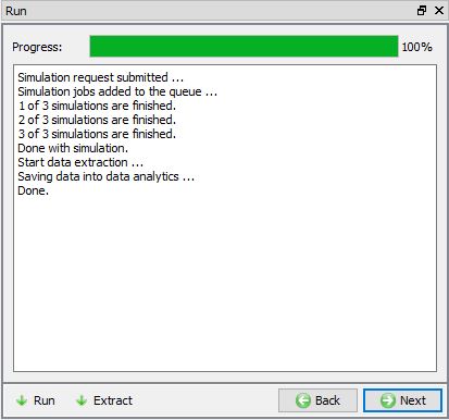
After completion of simulation, we can observe the Progress status as 100 %. Once the simulation completes, automatically data extraction will start to extract output (impact stress and residual stress output) from the simulated database and then exported to Data Analytics (DA model) file for further processing. Once the data extraction and exporting is completed, we can observe the message as “Done” (See Fig. STPL1.8.). By using option we can re-extract the data and save to DA model file. Click on to Impact stress page.

Run Options page to simulate 2D micro model

Run page showing status after completion of simulation

2D micro model impact stress and residual stress output

Once the simulation is completed, we can click on Impact stress or Residual Stress item in operation tree to view respective output from 2D Micro model. The Micro model simulation results can be displayed with contour plots and graphs.

Using , we can plot contours and using , we can plot graphs for Radial stress, Effective stress and Effective strain as shown in Fig. STPL1.9. and Fig. STPL1.10.

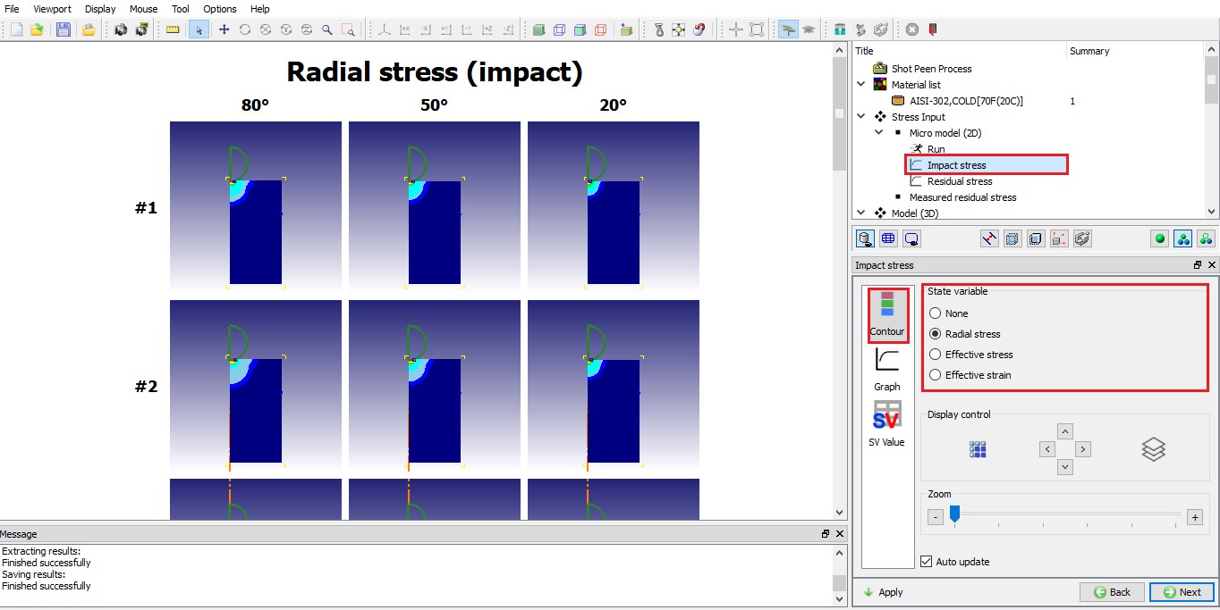
Radial impact stress Contour plot

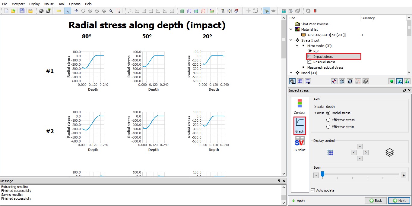
Impact radial stress along depth

Display of graphs and contour plots for multiple angles and multiple hits can be controlled using options available under Display control as shown in Fig. STPL1.11. User can select the range of data to be displayed using , in Fig. STPL1.11. hit #10 is selected to be displayed. (See Fig. STPL1.11.). The graph plots can be superimposed together to compare the results using as shown in Fig. STPL1.12.

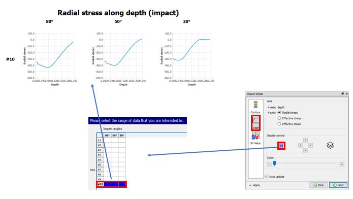
Selecting data range (Hit #10) of graphs display

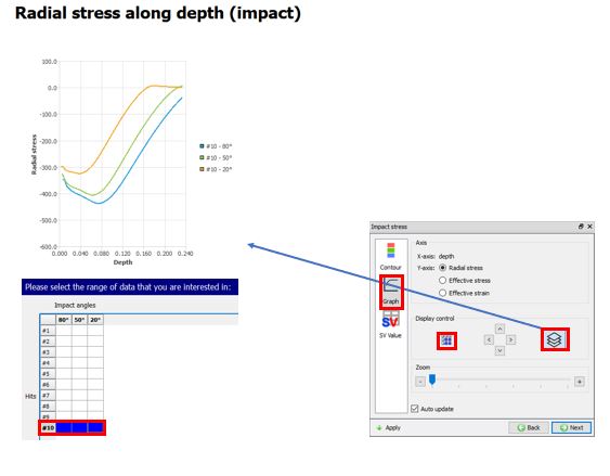
Super imposing graphs over one another for selected data range (Hit #10)

Using options, we can view Max radial stress, Max effective stress, Max effective strain, Dimple diameter and Dimple height state variables values either as Table or as Chart display depending on the selection in Display control. (See Fig. STPL1.13. and Fig. STPL1.14.).

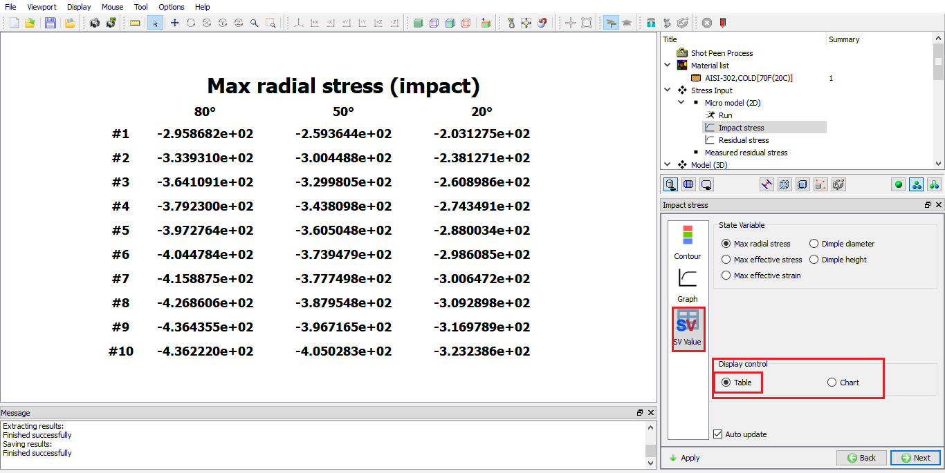
Max Impact radial stress values as table

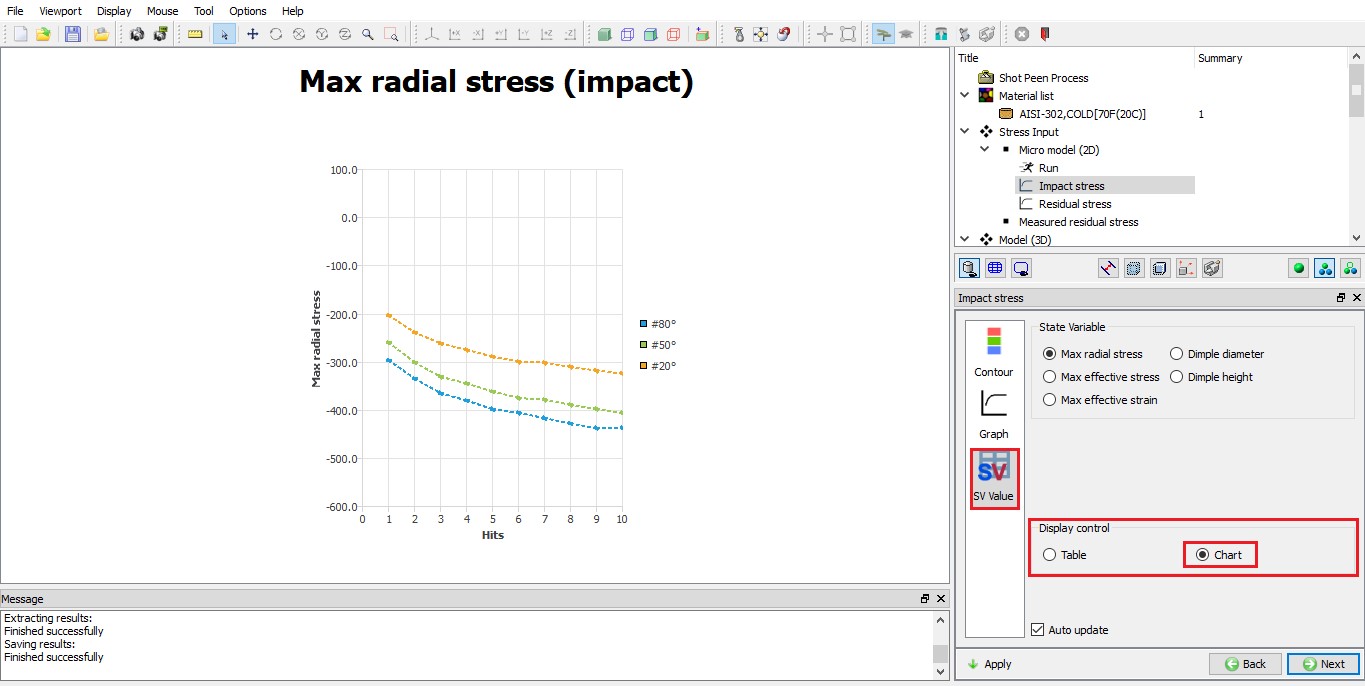
Max Impact radial stress values as Chart

Measured Residual stress

To provide measured residual stresses as input, click on “Measured Residual stress “ item in Object tree. We need to provide data for at least two impact angles. In this lab, we will define same measured residual stress values for both impact angles 90 and 20 as shown in Fig. STPL1.15.

Depth	Stress
0.0001	-93
0.00025	-95
0.0005	-72
0.00075	-50
0.001	-27
0.002	-11
0.005	0
0.01	0.2

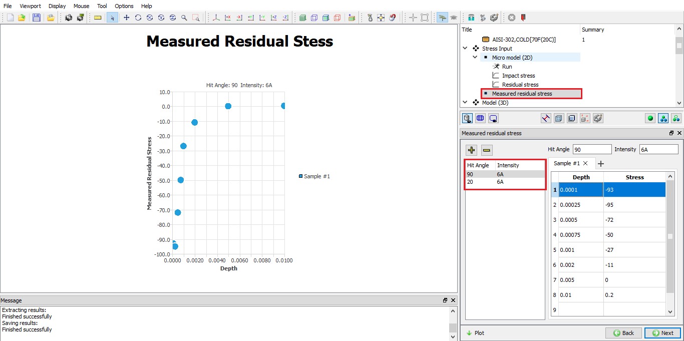
Input data of measured residual stress values

Defining 3D model for shot peening

Click on “Model3D ” item in object tree, in Model 3D page we can select the objects required to setup 3D model. In this lab, we require a Workpiece and one Nozzle object. By default one Workpiece and one Nozzle object will be selected, see Fig. STPL1.16. So, with default settings click to Workpiece page.

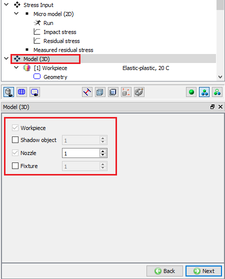
Defining required objects for 3D shot peening model

Defining Workpiece

Workpiece object page

In Workpiece page, keep the default object name as “Workpeice ” and click to Workpiece Geometry page.

Defining Workpiece geometry

Click on Import geometry from library and load Gear.stl from 3D/LABS/Shotpeening folder, imported Helical gear geometry looks like as shown in Fig. STPL1.17. Click until Workpiece Material page.

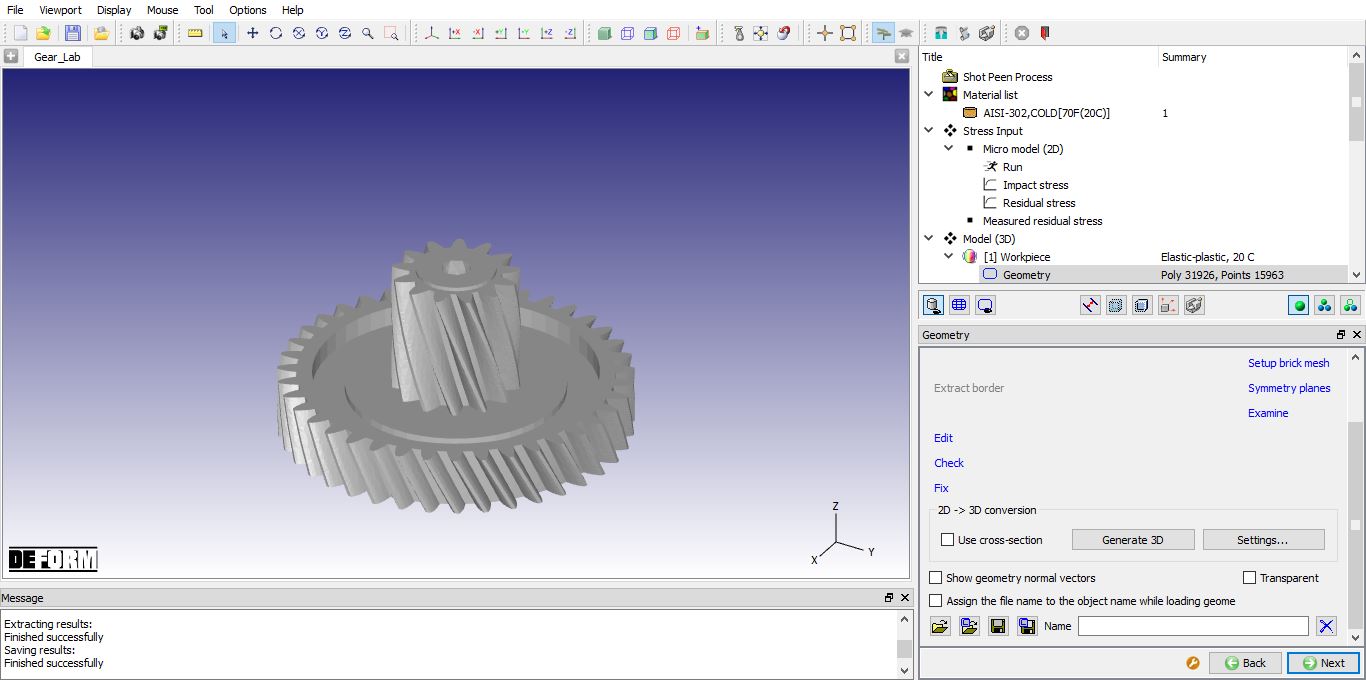
Imported Gear geometry

Defining Material for Workpiece

Assign “AISI-302,COLD[70F(20C)] ” material for workpiece, click button to generate mesh for workpiece.

Generating mesh for Workpiece

In Mesh page, define Target number of elements as 128000 and size ratio as 2. Click on Coating Tab, click on button to add 8layers and for each layer define coating thickness (micron) as 10 , then click on button to generate mesh. Click “Yes ” in “Generate coating mesh?” popup and “No ” in “Default Boundary condition” popup. Generated mesh for Workpiece is as shown in Fig. STPL1.19. Click till Boundary condition page.

Note : It is a good idea to check mesh after mesh generation. If a problem is detected, the mesh density may need to be decreased (make larger elements) or decrease the total coating depth. There is currently a limitation that the total coating depth can not be more than ½ the size of the smallest element.

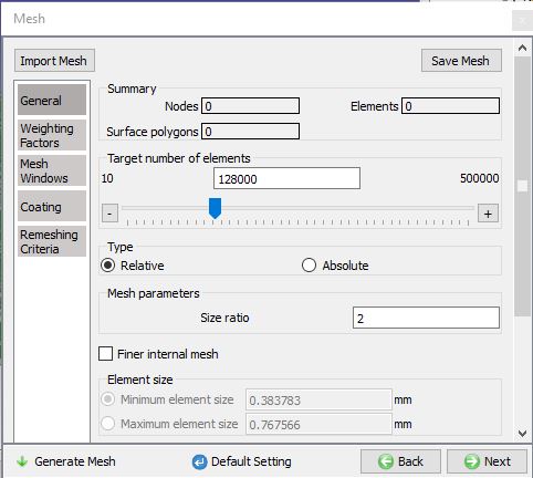
General mesh setting for workpiece

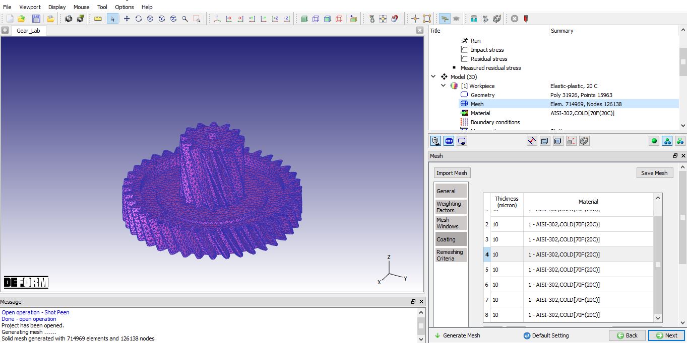
Coating mesh settings for Workpiece

Assigning boundary conditions to Workpiece

In this lab, we will fix the nodes on the bottom projection at the center of the gear as shown in Fig. STPL1.20. So, select Velocity option, pick the surface as shown in Fig. STPL1.20., then select “All ” direction radio button and click on button, assigned Velocity BCC for Gear object is as shown in Fig. STPL1.20. Click till Movement page.

Assigned Velocity boundary condition for Workpiece

Defining Workpiece movement

In Movement page, define Angular Speed as 10rpm. Define the center value as 0, 0, 0 and Axis value as 0, 0, 1 as shown in Fig. STPL1.21. Click till Nozzle #1 page.

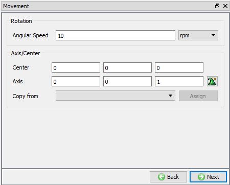
Workpiece movement page

Defining Nozzle #1

Nozzle#1 Object definition

For a nozzle, we can define name and its geometry in nozzle object page. In Nozzle #1 object page, we will keep the name as Nozzle # 1. We will define the Diameter as 5mm and Coneangle as 20 degrees, keep the massflow as 2.3 kg/min and Airpressure as 172 kpa as shown in Fig. STPL1.22. Click to Location page.

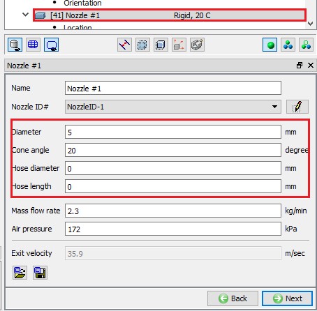
Defined Nozzle #1 parameters in object page

Defining Nozzle Location

Define Referenceco-ordinate X as 9.793 , Y as -12.395 and Z as 1.86717. Define Distance as 37mm , Theta as 61 degrees and Phi as 308degrees with respect to reference point as shown in Fig. STPL1.23. Click to movement page.

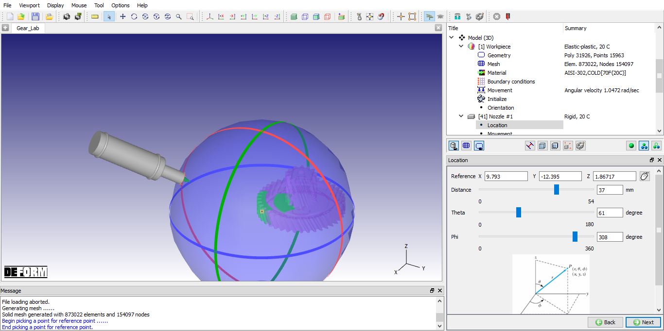
Defining Nozzle location

Defining Nozzle movement

Define nozzle Speed as 1 mm/sec and direction of movement as Z as shown in Fig. STPL1.24. Click to Positioning page.

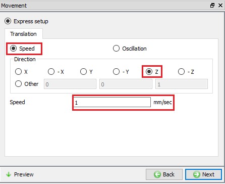
Defining Nozzle movement

Positioning

In positioning page, using we can position the object. In this lab, we need not use positioning as the Workpiece and Nozzle objects are in correct position.

Analysis of shot peening process

Shot peening process in 3D can be analyzed based on the stress input, process parameters and geometry of the objects.

Particle Simulation : During particle simulation, randomly generated particles hit the workpiece and calculates averages of impact angles, hit counts, impact velocities, etc. on each surface element. Particle simulation is slower than the Impact simulation and it handles ricochets.

Impact Simulation : During impact simulation, it performs simple cone intersections with workpiece and calculates impact angles, hit counts, impact velocities, etc. for each surface element. impact simulation is fast and does not consider impacts from ricochets. Also, it does not consider partial coverage of surface elements.

Residual stress Analysis : Impact stresses either from particle simulation or impact simulation can be assigned to the object for running the residual stress analysis to predict the residual stresses. If the stress input is only from Measured residual stress the residual stress analysis is not required, the Measured residual stress will be interpolated over the 3D model based on the Particle simulation output or Impact simulation output, depending on user selection.

Particle Simulation

Particle Simulation settings

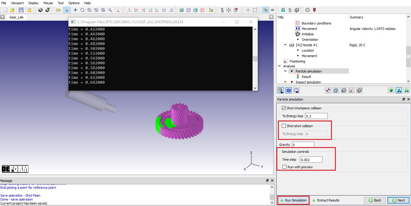
Click on “Particlesimulation ” item in Object tree. In this lab, we will define % of energy loss during Shot-Workpiece collision as 0.3. We will not shot to shot collisions, hence turn of Shot-shot collision check box. We will define time step as 0.002, too large time step may lead to shots penetrating the workpiece.

We can run simulation either with preview or without preview, if we run simulation with preview, the simulation will take more time, but we can observe the pellets striking the workpiece and if needed we can adjust the parameters by stopping the simulation. For this lab, we will run the simulation by turning off the Run with preview checkbox. Click on button, simulation will start running and current process time will be updated in console as shown in Fig. STPL1.25. Once the particle simulation is completed, click to results page.

Particle simulation settings

Particle Simulation Result

From particle, the following output parameters will be obtained:

• Vertical (normal to the surface element) velocity.

• Impact angle.

• Hit count.

• Hit density (hit count divided by surface element area).

• Exposure time.

• Coverage.

Click on “Result ” item under Particle simulation in Object tree. In Particle simulation results page, we can plot contour of different outputs along with histograms as shown in Fig. STPL1.26. Under State variable tab, we can plot contours of impact stress, residual stresses and measured stress state variables.

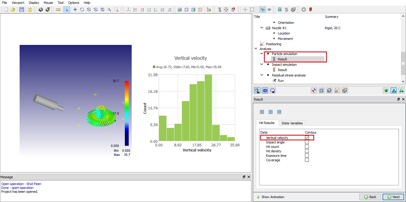
Vertical velocity histogram along with contour from particle simulation

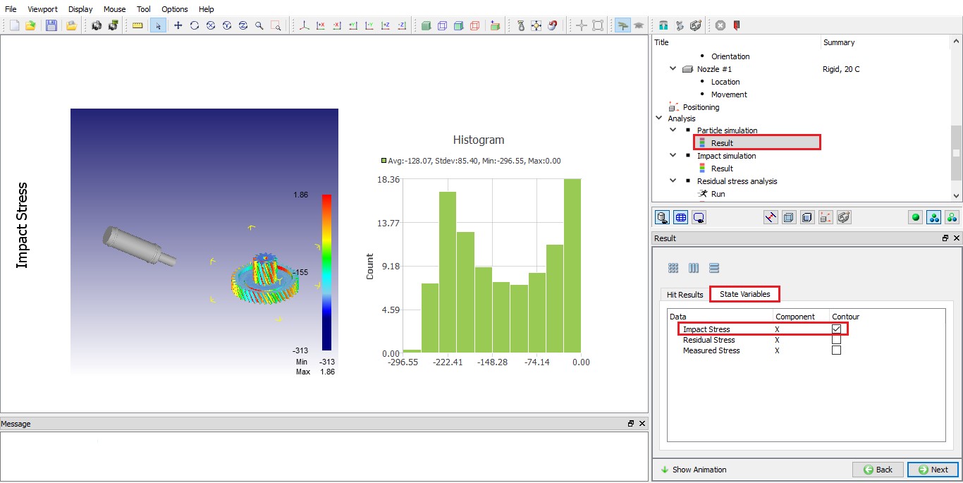
Impact stress histogram along with contour from particle simulation

We can view an animation of the particle simulation by clicking on action button.

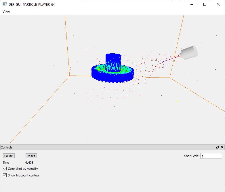
Particle simulation animation page

Impact simulation

Impact Simulation settings

Click on “Impactsimulation ” item in Object tree. In this lab, we will use default time step of 0.0333 sec. We can control the display of nozzle, nozzle cone and nozzle path but turning on/ off respective check boxes. Click on and observe the Impact simulation. In this lab, we will turn off all checkboxes. During impact simulation, we can observe the impact cone and path in the display and status in status bar, Determining hits : time on left side and total completion in percentage on right side. (See Fig. STPL1.29.). Click to impact simulation results page

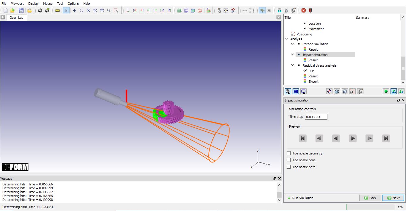
Impact simulation settings

Impact simulation result

Similar to Particle simulation results page, we can plot contour of different Hit results along with histogram as shown in Fig. STPL1.30. and Fig. STPL1.31. Under State variable tab, we can plot contour of Impact stress, Residual stresses and Measured stress State variable output. Click to Residual stress analysis page

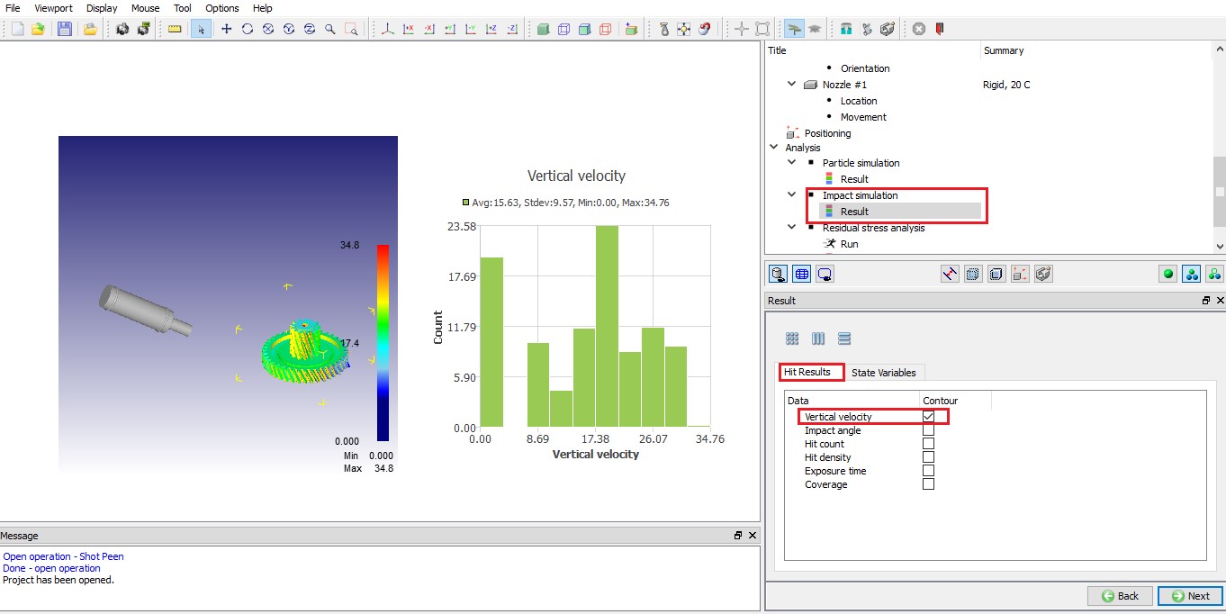
Vertical velocity histogram along with contour from impact simulation

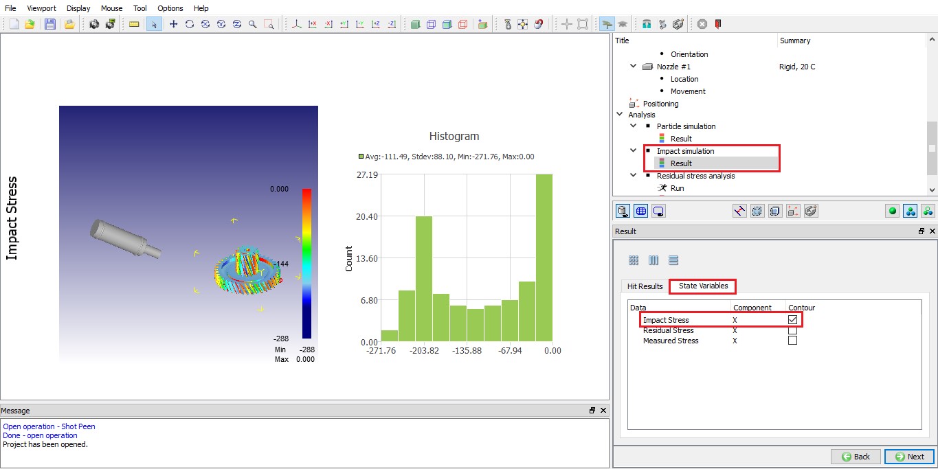
Impact stress histogram along with contour from Impact simulation

Residual stress analysis

Residual stress analysis settings

In residual stress analysis page, we can assign initial impact stress values either from Particle simulation or Impact simulation to the workpiece. In this lab, we will select Impact simulation radio button and click on Assign Initial stress button. With “MUMPS “ as solver, click on and then click on the button to generate the database (See Fig. STPL1.32.) Once the database is generated click to the Run page.

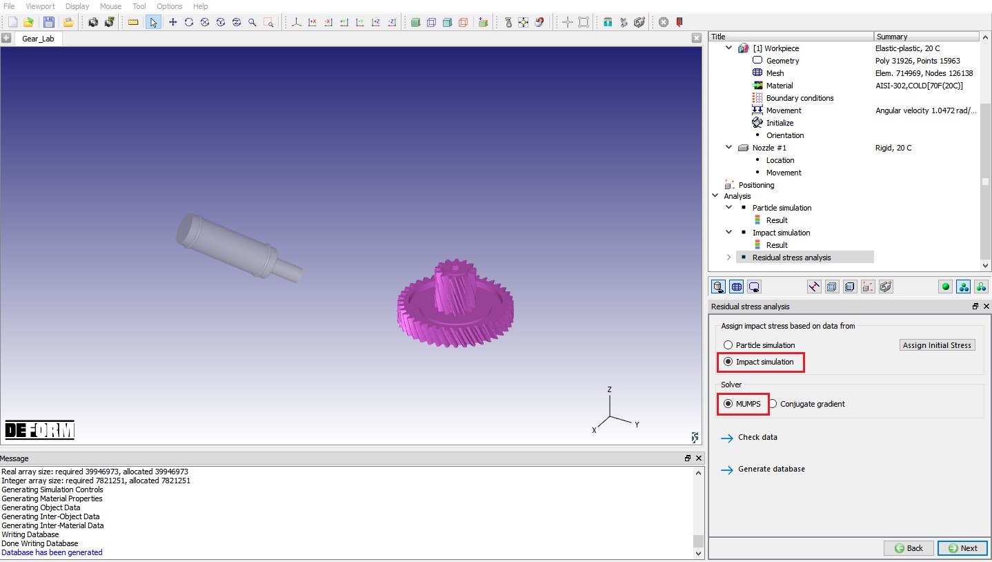
Residual stress analysis settings

Simulating Residual stress analysis

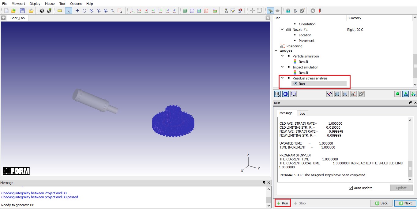
Click on to run single step FEM stress re-equilibrium simulation (Residual stress analysis) simulation. Once the simulation is completed, click on to Results page. Fig. STPL1.33. Shows end of residual stress analysis.

Residual stress analysis Run page

Residual Stress analysis results

In results page, we can plot contours for selected output, Fig. STPL1.34. Shows Effective residual stress contour plot.

Residual stress (FEM) – Calculated from FEM simulation based on the Impact/ Particle simulation

Residual stress (from micro model) – Residual stresses from 2D micro model are interpolated onto 3D model based on the Impact/ Particle simulation

Impact stress (from micro model) – Impact stresses from 2D micro model are interpolated onto 3D model based on the Impact/ Particle simulation

Measured stress - Residual stresses from the measured data provided by the user are interpolated onto 3D model based on the Impact/ Particle simulation

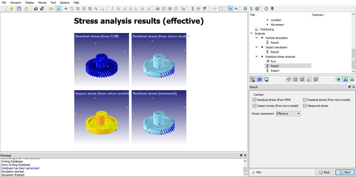
Effective stress output for different outputs Micromodel, Measured stress and FEM