Steady State Extrusion Lab1

In this Lab we are setting up a simple operation of Steady state extrusion by importing a DB of the ALE Extrusion lab (3D_ALE_EX_Lab1) . We will also use bearing length adjustment in this Lab.

The application of this lab will extrude 5 small cylinder parts from a large cylinder billet. The model of the workpiece used in ALE is with symmetry as shown in Fig. SSEXTL1.1. The diameter of D0 is 140 mm. The diameter of D1 is 26 mm. The diameters of D2 and D4 are 27 mm. The diameters of D3 and D5 are 28 mm.

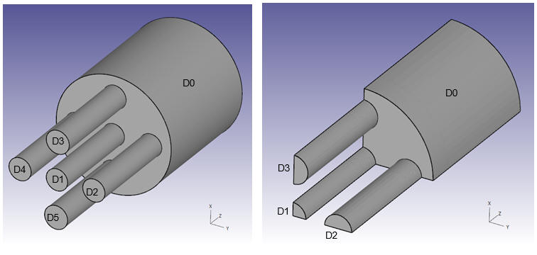
Model of the Workpiece

1.1. Creating a New Problem

1.2. Adding Operation

1.3. Importing ALE Extrusion Database

1.4. Simulation Setup

1.5. Step Controls

1.6. Generate DB

1.7. Running Simulation

1.8. Post Processing

1.9. Bearing Length Adjustment

1.10. Comparisons of simulation results

Creating a New Problem

On a Windows machine , go to the button select DEFORM-v1x.xxx (.xxx indicates version number E.g. v14.0.2) and select DEFORM GUI Main vxx.xx from the menu. The DEFORM GUI Main window will appear as shown below Fig. SSEXTL1.2.

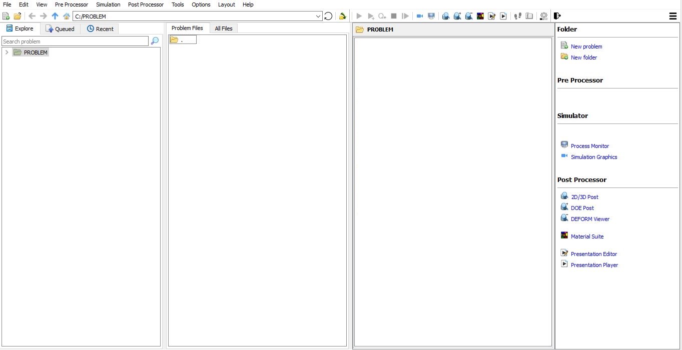
DEFORM GUI Main window

Create a new problem either by selecting File New Problem or by clicking the New Problem icon. The Problem Setup window will appear as shown in Fig. SSEXTL1.3. Select “Integrated Manufacturing Process “ radio button and unit system as “SI “ radio button in unit field. Define Problem Name as “****3D_SS_EX_Lab1** ” and make sure the “Show option dialog** ” check box is turned on (if we do not turn on the “Show option dialog ” check box, then we will not get the New Project dialog in MO UI). Then click on button to open a new Problem using the Deform Integrated Manufacturing Process.

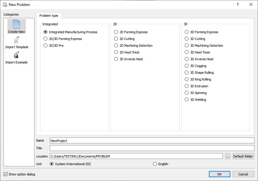
New Problem page

Multiple operation wizard will open with the New Project dialog, at this point user will be prompted to specify a project name (system will create a separate folder with this project name) and title for this session. In this session we will use “3D_SS_EX_Lab1 “ as the project name. Click on to continue to open the operation.

Adding Operation

Add 3D Extrusion operation from the Explorer Operations list. Add the operation by clicking on button available next to 3D Extrusion or user can also add by drag and drop into the Operation Editor. When we add the 3D Extrusion operation, process settings Window will open by default.

Importing ALE Extrusion Database

At this point, we can import the first step from the ALE database (Database generated in ALE Extrusion Lab1 (3D_ALE_EX_Lab1) setup). Click File **Import** , select 3D_ALE_EX_Lab1.DB and choose Step -1. Now we just need to change the things that are different between the ALE simulation and the new Steady State analysis.

Simulation Setup

Go to Simulation setup , and choose Steady state extrusion radio button in Simulation method. Set the Strain update and Temperatureupdate with 0 per step in Acceleration, then uncheck the Strain update and Temperatureupdate check boxes. Simulation setup is shown in Fig. SSEXTL1.4. Click on until Step controls or choose Step Controls from Operation tree.

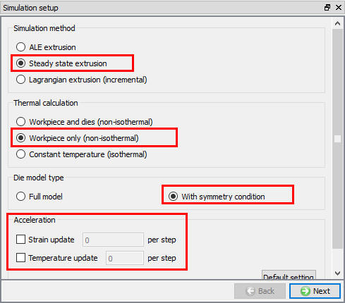
Simulation setup

Step Controls

Click to switch to expert mode in the top menu bar for step control.

Simulation steps

In the simulation of Steady state extrusion, the geometry will be updated only at the last step based on the calculated velocity field.

If we define contact separation relationship between workpiece and the die with ‘Non-separable’, the velocity field will reach the steady state after 2 simulation steps. In this situation, 5 steps of simulation are enough for Steady state extrusion.

If we define contact separation relationship between workpiece and the die with ‘Separable’, there will be separation and contacting in the bearing region at every simulation step. So, we need more simulation steps for the velocity field to reach the steady state. In this situation, 10 steps of simulation are generally enough for Steady state extrusion.

So, in this lab, we set Numberof simulation steps as ‘5 ‘ and StepIncrementto save as ‘1 ‘ in the Simulation steps dialog (see Fig. SSEXTL1.5.).

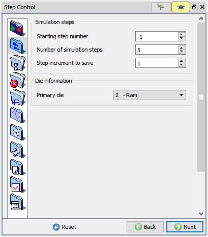
Simulation step setup

Stop criteria

In the Stopcriteria dialog, click the ALE Steady State page, uncheck ‘Turn on steady-state stop control ‘ if not unchecked (see Fig. SSEXTL1.6.).

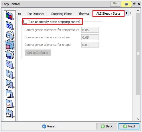
Stopping control

Generate DB

Then go to Generate DB page. Click to see if anything was missed in the setup and then click on the button to generate the database. Observe the message in Message tab informing database generation status.

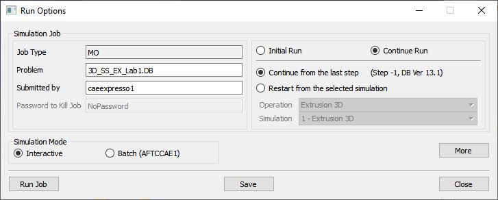
Running Simulation

Once the database has been generated switch to the Simulation mode by clicking on button above the operation tree. Click on the action label to open the Run Options dialog as shown in Fig. SSEXTL1.7.. Use the default ContinueRun option to select “Continue from the last step ” (from step -1) option and then select the Simulation mode as Interactive radio button. Click on button to run the simulation.

To define MPI settings, click on button, Run Options window will expand and displays options to define MPI settings for simulation (max number of processors that can be defined depend on your 3D MPI license).

Run Simulation Window

Monitor the progress of the simulation by looking at the Simulation Message and Simulation Log tab, make sure that the option is checked. User can view the Extrusion process from Simulation graphics as the simulation proceeds to the specified Step definition.

Post Processing

When the simulation is completed, review the results by switching to Post mode using the button above the Simulation tool bar.

Plots of the EffectiveStrain and Temperature of the workpiece at last step are given in Fig. SSEXTL1.8. and Fig. SSEXTL1.9.

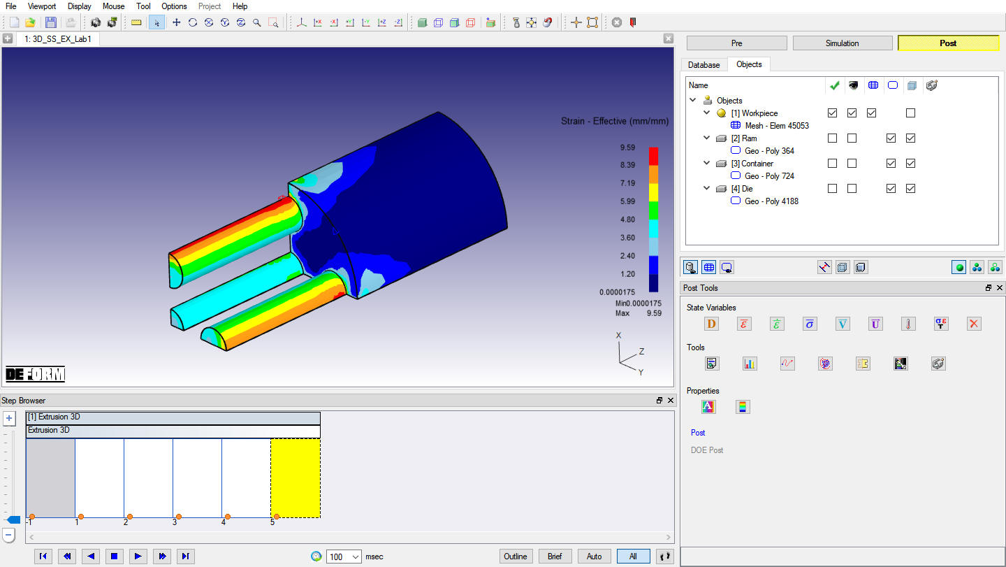
Effective Strain distribution at last step

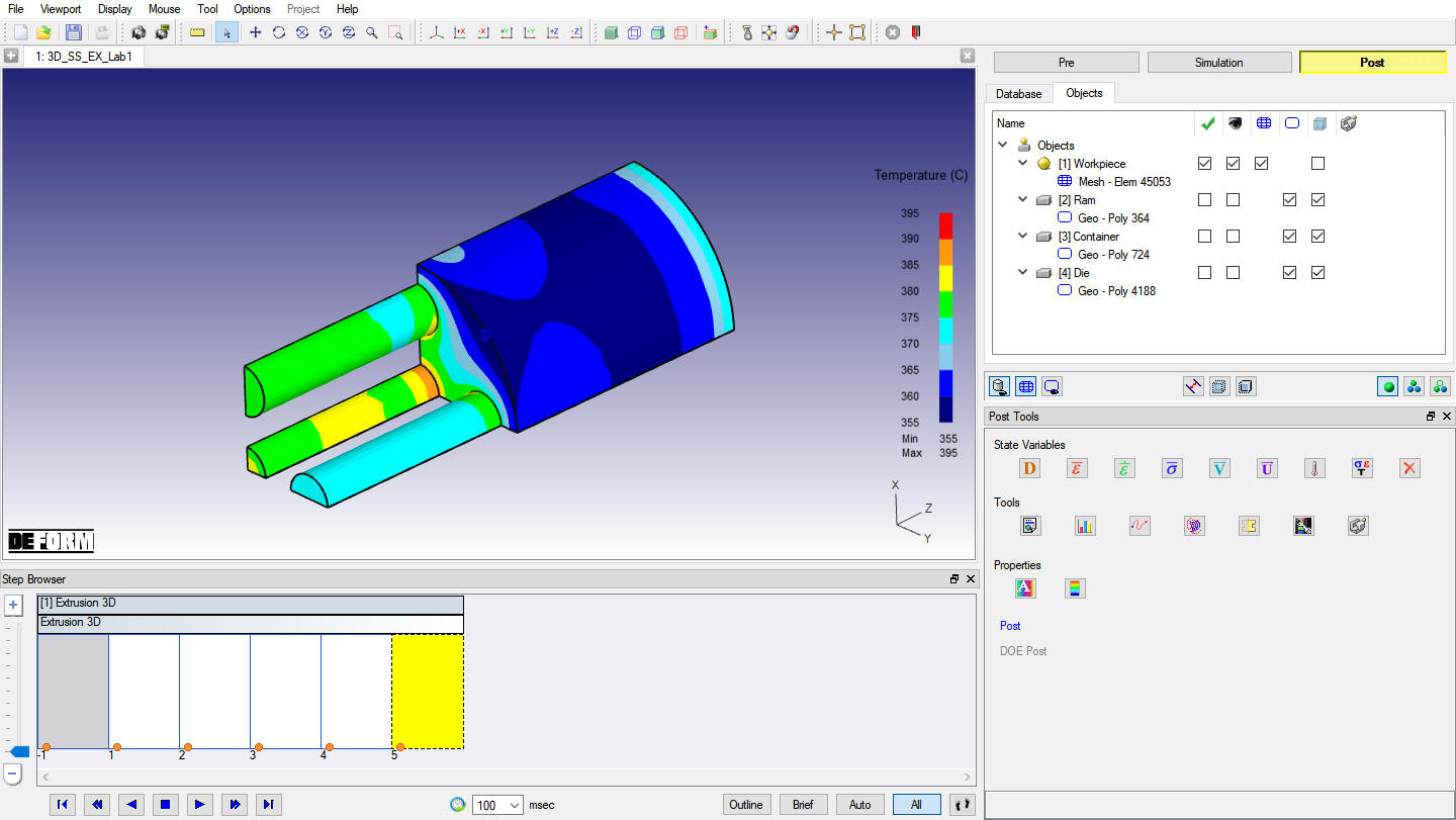
Temperature distribution at last step

Plot of the X displacement and Y displacement of the workpiece at last step is given in Fig. SSEXTL1.10. and Fig. SSEXTL1.11. Even though the displacements are very small we cannot observe the shape bending, but from the displacement distribution in X direction, we can see the dominated displacement is located at profile D3 with negative value. From the displacement distribution in Y direction, we can see the dominated displacement is located at profile D2 with negative value. This concludes that surround profiles (D2 & D3) bent toward the central profile (D1) after extrusion, which is similar to the simulation result of Lagrangian extrusion.

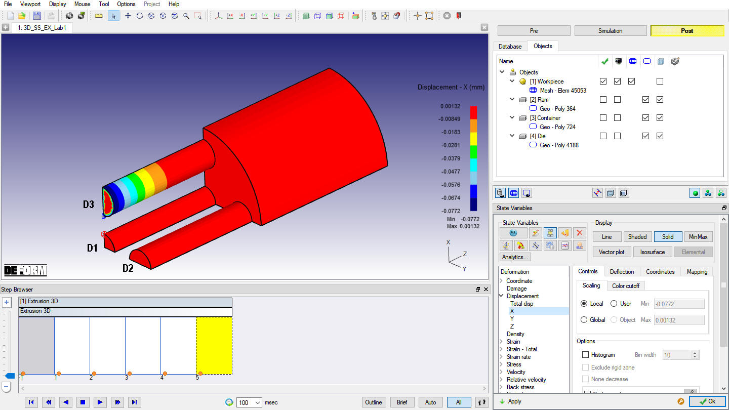
X- Displacement distribution of the workpiece at last step

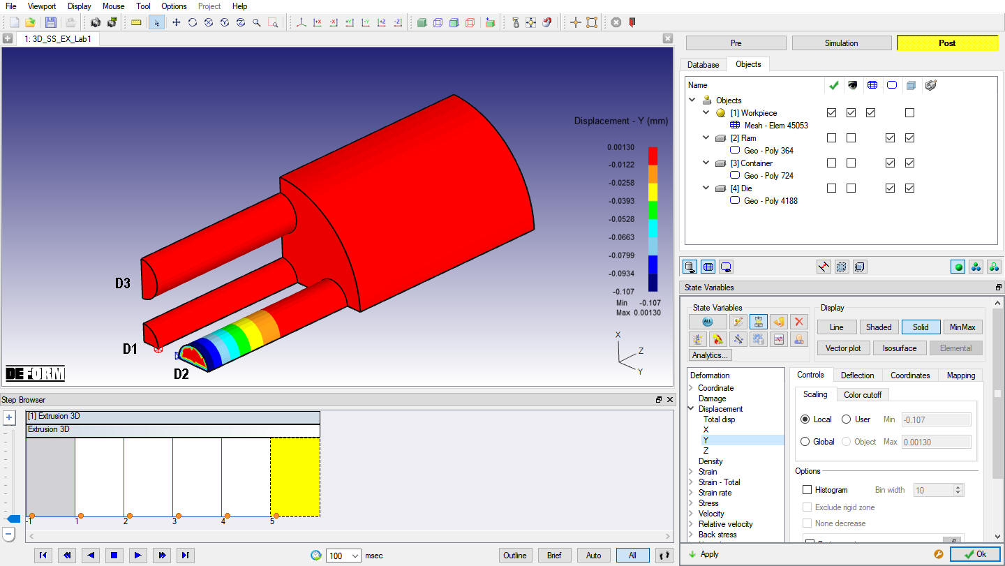
Y-Displacement distribution of the workpiece at last step

Bearing Length Adjustment

In extrusion, bending, wrap and twist of profiles are mainly caused by the unbalance material flowing. In this example, for surround profiles, the material of outer side flew faster than that of inner side, which caused the bending. We can use bearing length adjustment to reduce the bending of surround profiles.

We should keep the simulation set up and simulation result of this project and do the simulation of bearing length adjustment with another project.

Simulation step up of bearing length adjustment

In File menu, click on New and click on in both Questions popups, new Project will be open with New project popup.

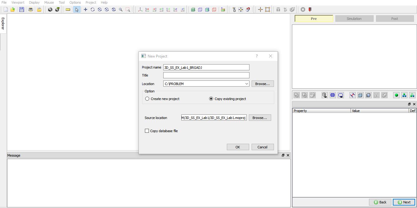
In New Project popup define the Project name as “3D_SS_EX_Lab1_BRGADJ “, select Copyexisting project radio button, click on browse and browse “ 3D_SS_EX_Lab1 “ project and click on in New Project popup. The “ 3D_SS_EX_Lab1” project is copied into “3D_SS_EX_Lab1_BRGADJ “ along with all settings.

New Project for bearing length adjustment lab

Go to Die **Die Bearing Control Points** page.

In this lab, we will reduce the inner side bearing length of profile D2 to speed up the material flowing on this side, and increase the outer side bearing length of profile D3 to slow down the material flowing on that side.

In the DieBearingControlPoints page, select bearing surface 1 (highlighted with green color in display window), define 3 control points by clicking on the bearing entry edge at positions of inner side, middle and outer side. Then we can edit their coordinates and length scales in the control points table. Select point 1 in the table, change its coordinates to (0,31.5,0), change its Length Scale to ‘0.55’. Select point 2 in the table, change its coordinates to (13.5,45,0), keep its Length Scale as ‘1’. Select point 3 in the table, change its coordinates to (0,58.5,0), keep its Length Scale as ‘1’. We can see the bearing shape and bearing length for surface 1 are changed (see Fig. SSEXTL1.13.).

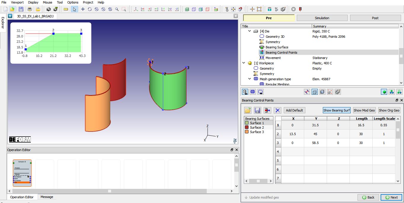
Control points setting of bearing surface 1

Select bearing surface 3 (highlighted with green color in display window), define 3 control points by clicking on the bearing entry edge at positions of inner side, middle and outer side. Then we can edit their coordinates and length scales in the control points table. Select point 1 in the table, change its coordinates to (31,0,0), keep its Length Scale as ‘1’. Select point 2 in the table, change its coordinates to (45,14,0), keep its Length Scale as ‘1’. Select point 3 in the table, change its coordinates to (59,0,0), change its Length Scale to ‘1.5’. We can see the bearing shape and bearing length for surface 3 are changed (see Fig. SSEXTL1.14.).

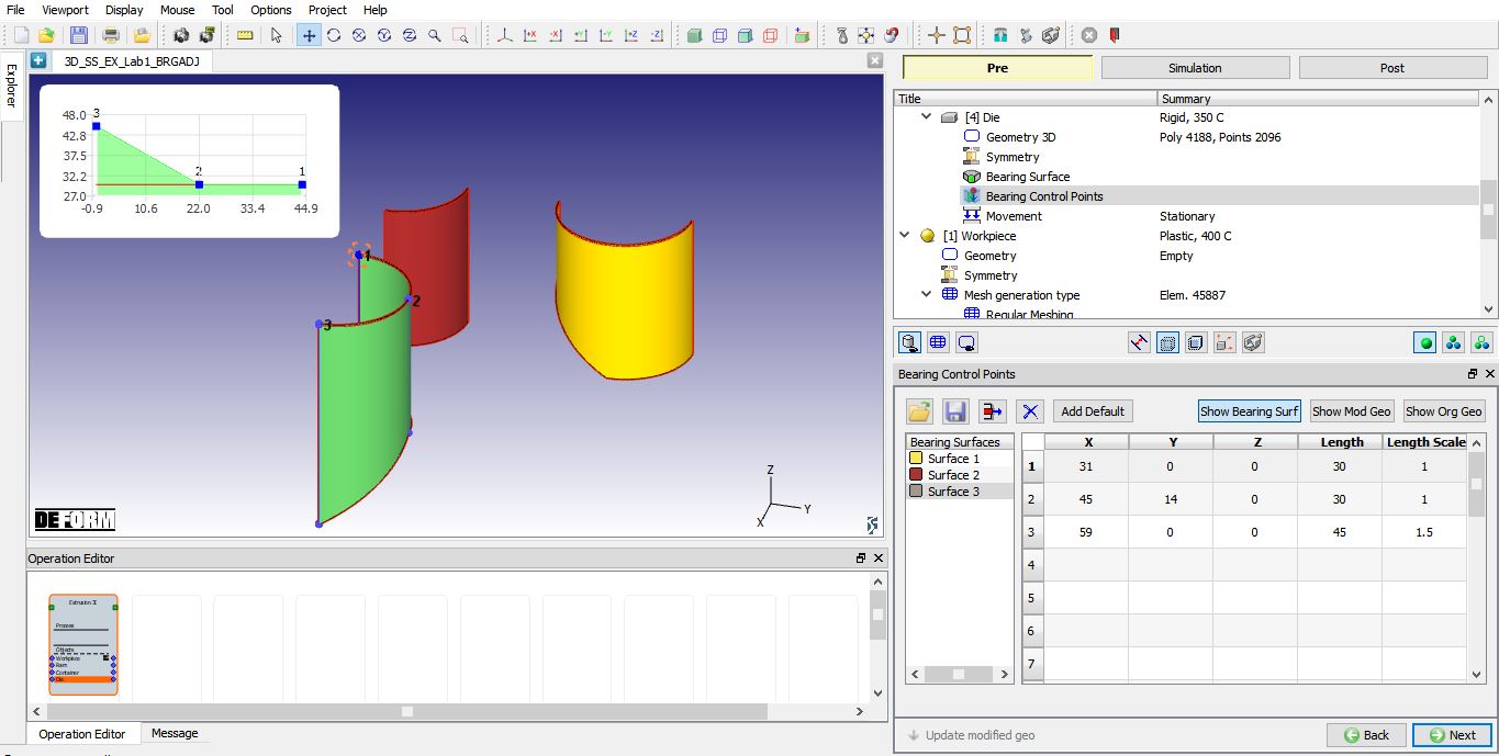
Control points setting of bearing surface 3

Click in the Die Bearing Control Points page, rotate the object in the Display window, we can see the modified die geometry in Fig. SSEXTL1.15.

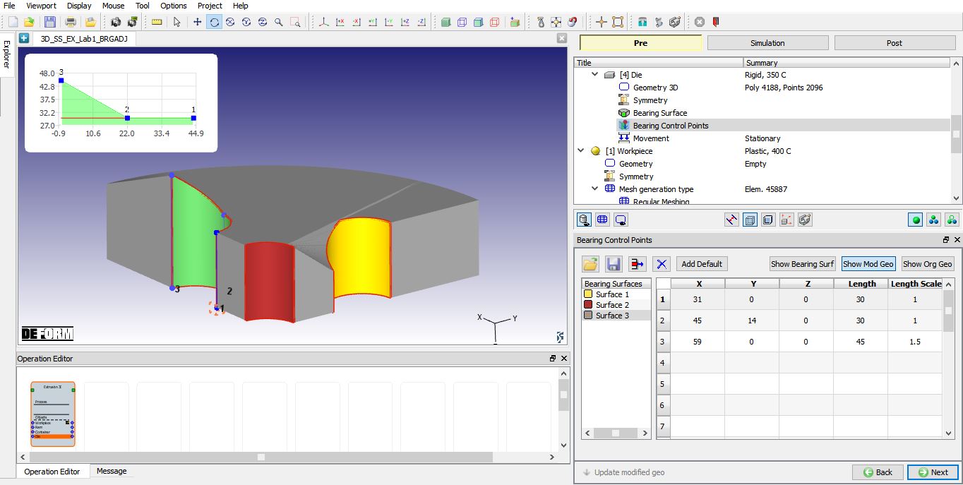
Die geometry after bearing length adjustment

Go to Step Control page, in the Stop criteria dialog, click the ALESteadyState page, uncheck ‘Turn on steady-state stop control ‘ (see Fig. SSEXTL1.6.).

Generate DB

Running Simulation

Once the database has been generated switch to the Simulation mode by clicking on button above the operation tree. Click on the action label to open the Run Options dialog as shown in Fig. SSEXTL1.16. Use the default ContinueRun option to select “Continue from the last step ” (from step -1) option and then select the Simulation mode as Interactive radio button. Click on button to run the simulation.

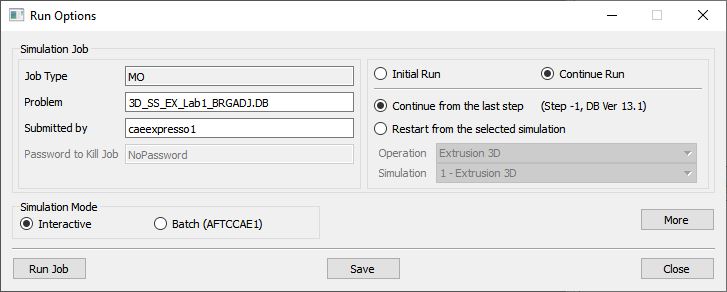
Run Simulation Window

Monitor the progress of the simulation by looking at the Simulation Message and Simulation Log tab, make sure that the option is checked. User can view the Extrusion process as the simulation proceeds to the specified Step definition from Simulation graphics.

Comparisons of simulation results

After the simulation of modified bearing surface is completed, we can compare the simulation results in Post processor.

In DEFORM GUI Main window, highlight “3D_SS_EX_Lab1.DB “, then click to open “3D_SS_EX_Lab1.DB “ in Post processor.

In Post-processor, from the top menu bar, click File **Open** , select “3D_SS_EX_Lab1_BRGADJ.DB “, then click .

From the top menu bar, click Windows**Tile Vertically** , we can see that both “3D_SS_EX_Lab1.DB “ and “3D_SS_EX_Lab1_BRGADJ.DB “ are opened in Post processor. Thus, we can compare the simulation results of 2 databases in the same display window.

In the display window, with the right mouse, both check ‘DB Info ‘ and ‘Title ‘ to display the name of database and the simulation step.

Firstly, we compare the contacts of the workpiece at last step. We can obviously see the different contacts in surround profiles D2 & D3 after their bearing length adjustments (see Fig. SSEXTL1.17.).

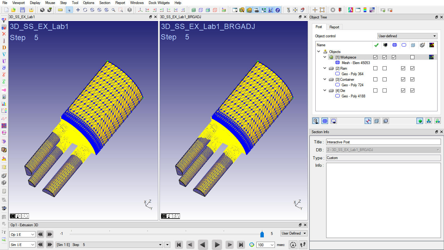
Contacts comparison of the workpiece at last step

Then, we compare the displacements. Comparison of X-Displacement of the workpiece at last step is given in Fig. SSEXTL1.18. We can see the dominated displacement in X direction marked with Min value reduced to 20% after bearing length adjustment.

Comparison of Y-Displacement of the workpiece at last step is given in Fig. SSEXTL1.19. We can see the dominated displacement in Y direction marked with Min value reduced to 40% after bearing length adjustment.

So, bearing length adjustment is an effective method to change the balance of material flowing for ALE & Steady state extrusion.

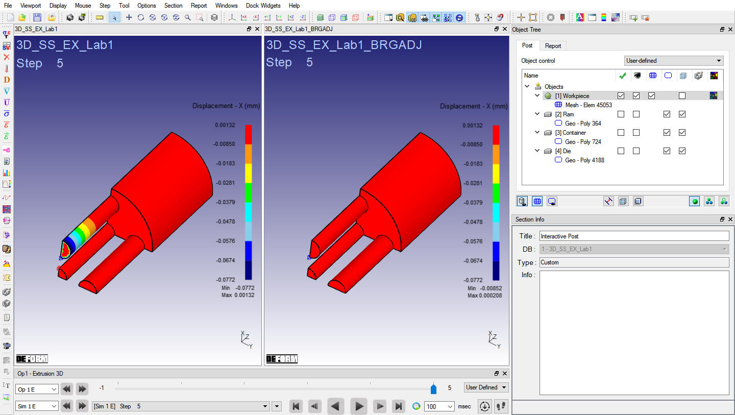
X-Displacement comparison of the workpiece at last step

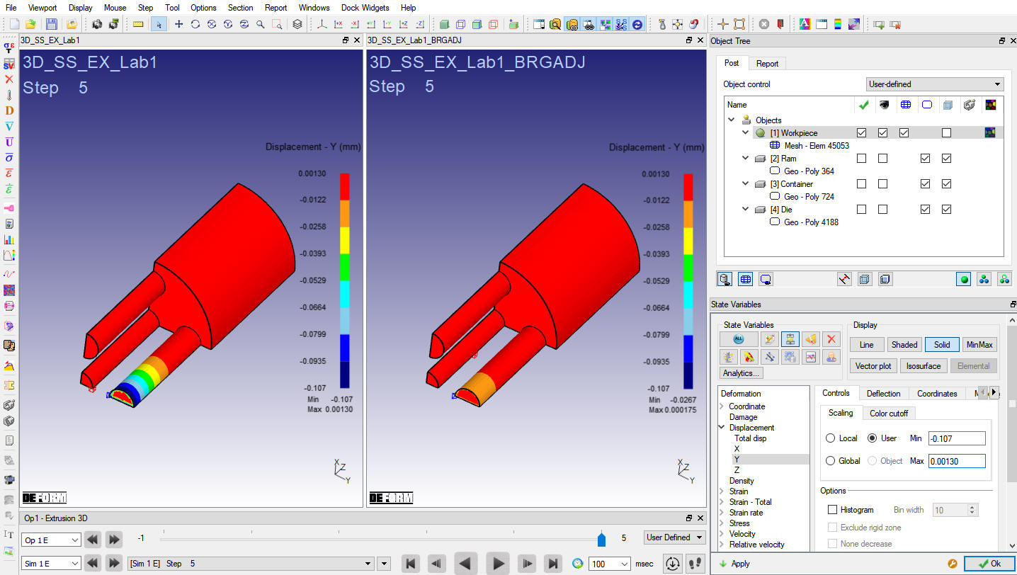
Y-Displacement comparison of the workpiece at last step