Appendix V: The elasto-plastic model

AV.1. Material Properties

AV.2. Object data

AV.3. Solution procedure

AV.4. Strain Definition

AV.5. Advice on Predicting Springback

AV.6. Note on Convergence issues with Elasto-Plastic material models

AV.7. DEFORM convention rule for material interpolation

AV.8. Comments on “Flow curve definition for Rate-dependent material”

In general, the elasto-plastic material model should be run in a very similar manner as the rigid-plastic material model. Some differences are discussed in the following section.

Material Properties

In addition to the flow stress data, the material is also required to have Young’s modulus (YOUNG) and Poisson’s ratio (POISON). If thermal expansion and contraction is to be considered, the thermal expansion coefficient must also be present. Note: elastic and elasto-plastic materials in DEFORM deal with thermal expansion differently (see Thermal expansion (EXPAND) for more details).

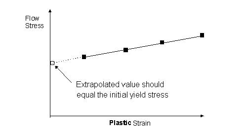
In the elasto-plastic model, the flow stress at zero strain represents the yield stress for the material. As the accumulated effective plastic strain increases, the yield stress increases. The flow stress data must have a reasonable description for the initial yield stress particularly in the case of low deformation simulations such as heat treatment. This is where the elastic part of the stress-strain curve intersects with the plastic part of the curve. If the flow stress data is only defined for high strain values, DEFORM will extrapolate the yield stress and this value may not be close to the actual yield stress. Thus, valid results are unlikely and convergence difficulties are possible. Thus, having some flow stress data at low effective plastic strain values may aid convergence. (See Fig. AV.1 for an example of extrapolation of the initial yield stress).

In order to provide guidance to users who are not familiar with modeling elasto-plastic materials, we offer the following suggestions.

1. When using the function form (Power law):

|
—|—

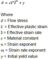it is accurate for ‘y’ to be equal to the initial yield stress. If y = 0, the initial yield stress will be poorly represented.

2. When using a table form, the program will extrapolate/interpolate the flow stress and use that as the initial yield stress. If extrapolation is expected, be sure that the slope of the flow stress in the small strain region is “reasonable”, i.e. extrapolated value should be the same as the initial yield stress. Some modifications may be needed in the small strain region, like adding one more point to correct the slope. These modifications should be made even if the flow stress is retrieved from the DEFORM material database.

Extrapolation of flow stress data to determine the initial yield stress

Object data

Set the EP initial guess under Objects/Properties/Deformation to Previous step solution.
If there is a change in operation, e.g. moving the part from one station to another, initialize the velocity for the part under Objects/Nodes Data/Deformation. This will improve the initial guess of the velocity solution.
If moving the part from one set-up to another, allow the part to relax its stresses by placing a few springback steps between operations.

Solution procedure

Always use Newton-Raphson iteration method or BFGS iteration method. The user can select the different methods under Simulation Controls/Iteration. It is useful to try switch iteration methods when either one fails to converge.
The force error norm can be increased two orders of magnitude larger than the velocity error norm. This is suggested only when the solution fails to converge due to non-stationary force error norm behavior. The value can be changed under Simulation Controls/Iteration (Convergence Error Limit)
It is recommended to reduce the value after convergence has been achieved.
Elasto-plastic convergence is very sensitive on time-step size. By selecting a time step size too large (size depends on the simulation), convergence may be very difficult. By reducing time-step, convergence in many cases may be improved.

Strain Definition

The calculated strain components are of the “plastic” strain and the “effective strain” is the effective plastic strain.

Advice on Predicting Springback

To calculate the residual stress or springback during unloading, one of two methods may be used.

If the amount of springback or residual stress is the chief concern, remove the dies, put enough constraint on the workpiece to prevent rigid body motion. run a one step simulation.

If the user wishes to observe the material response during the unloading, then reverse the direction of the primary die. run multiple small steps.

Note on Convergence issues with Elasto-Plastic material models

Background : It has been a common and convenient approach for the users to use the material data from an existing model or from library data. As long as material data covers the range experienced by material point for a given simulation the model behavior is generally smooth. But once this material point crosses the defined data range, it is important to note that the flow stress data extrapolation plays a role in the accuracy of the model results. This becomes even more critical for elasto-plastic models when we need to depend on these extrapolated data to compute material yielding. This note summarizes couple of important points in this regard.

As the example shows in the Appendix, Log interpolation may lead numerical difficulties for some material data. In order to get more stable results, new convention rule is introduced in V6.1.

DEFORM convention rule for material interpolation

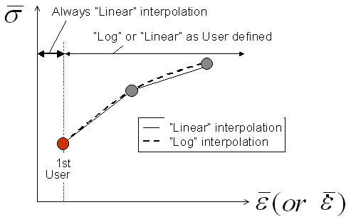
Convention: See Fig. AV.2.

If the current plastic strain is smaller than the 1st data point user defined, then “Linear interpolation” will be used.
If the current plastic strain rate is smaller than the 1st data point user defined, then “Linear interpolation” will be used.

Convention rule for flow stress definition

Note :

If the user doesn’t want to use the convention rule, the user should specify zero strain and zero strain rate curves.

Comments on “Flow curve definition for Rate-dependent material”

Typical convergence issues related elasto-plastic objects are related to material data and “material instability”. It may lead to the failure in “material routine convergence” and can potentially give wrong stress predictions. Here the flow curve definition for Rate-dependent material will be discussed briefly.

Material AISI-1010, Cold (Log interpolation): The general shape of curve looks like “Hardening material”. Two curves at different strain rates ( = 1 , 100) defined. (See Fig. AV.3.)

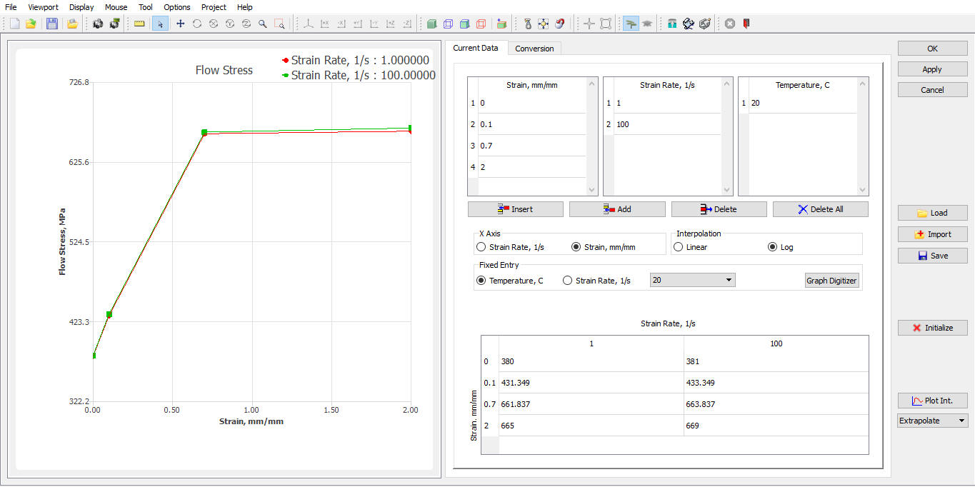
Flow curves for “AISI-1010,Cold”

Special care is needed in using LOG interpolation

User can choose one of interpolation methods, either “Log” or “Linear”. When user choose “Log (default)”, the interpolated curve at the small strain rate (= 0 ~ 1) is shown in Fig. AV.4. The curve at the zero strain rate now has softening behavior.

(“Linear interpolation results” is still hardening behavior as shown in Fig. AV.5.)

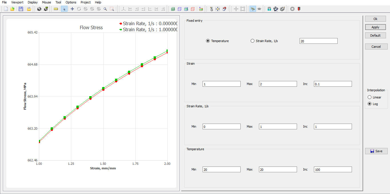
Log interpolation at the small strain rate(= 0 ~ 1)

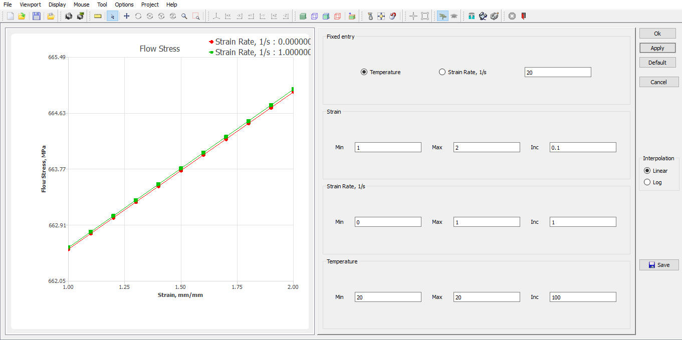
Linear interpolation at the small strain rate(= 0 ~ 1)

Related Topics: