31.1. 3D Extrusion
31.1.1. How to add the 3D Extrusion Operation
31.1.2. Simulation setup
31.1.3. Material List page
31.1.4. Defining Extrusion Dies
31.1.5. Die Object Page
-
Geometry
-
Symmetry
-
Dies Mesh Page
-
Material Selection
-
BCC Page
-
Movement
-
Bearing surface
-
Bearing Control Points
31.1.6. Defining Extrusion Billet
-
Workpiece Geometry Page
-
Workpiece Mesh Generation Type
-
Workpiece BCC Page
-
Property
-
Initialize
-
B.I. Flownet
31.1.7. Controls
31.1.8. Contact
31.1.9. Step Controls
31.1.10. Generate DB
How to add the 3D Extrusion Operation
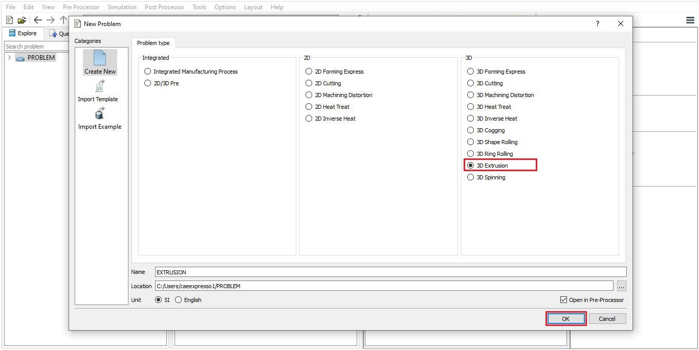
Extrusion operation can be setup in Integrated Manufacturing Process environment that can be accessed from GUI Main. User can create a new problem by either selecting File ![]() New Problem or by clicking the New Problem
New Problem or by clicking the New Problem ![]() icon, select 3D Extrusion radio button under problem type and unit system and then click
icon, select 3D Extrusion radio button under problem type and unit system and then click ![]() button as shown in Fig. 31.1.1. Integrated Manufacturing Process wizard will open, we can see that 3D Extrusion operation is added in Operation editor.
button as shown in Fig. 31.1.1. Integrated Manufacturing Process wizard will open, we can see that 3D Extrusion operation is added in Operation editor.
Adding Extrusion operation using GUI Main
We can also add Extrusion operation into Integrated Manufacturing Process environment from the New Project pop-up when a new problem is opened in Integrated Manufacturing Process environment as shown in Fig. 31.1.2. Using “Copy Existing project” option, we can import previous saved projects as new project from the New Project pop-up.
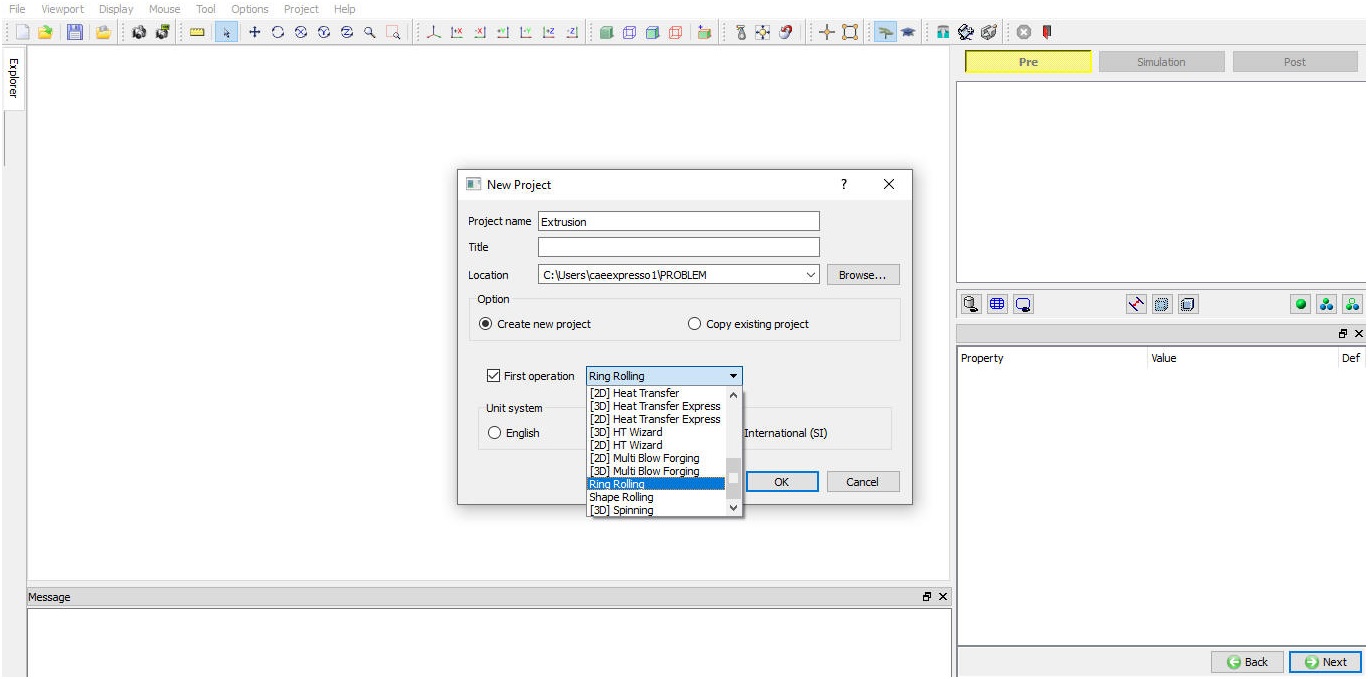
Assign Project name and First Operation selection in New Project window
We can also add Extrusion operation to operation editor from explorer tab in Integrated Manufacturing Process environment, by clicking on ![]() button next to Extrusion operation as shown in Fig. 31.1.3. or by drag and drop Extrusion operation into operation editor window.
button next to Extrusion operation as shown in Fig. 31.1.3. or by drag and drop Extrusion operation into operation editor window.
As the Extrusion operation is added into operation editor Simulation setup selection page will be opened in property settings modification window.
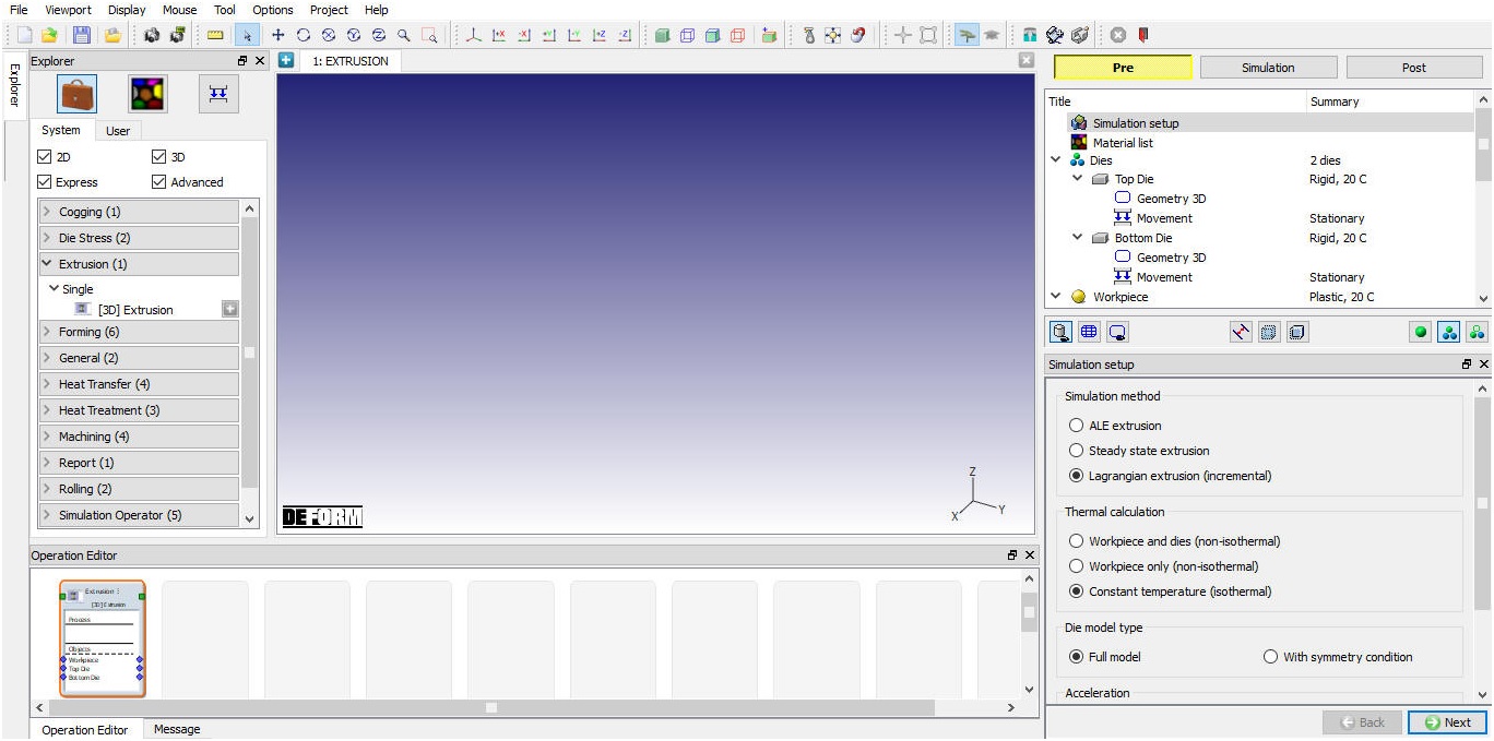
Adding operation from Explorer Operation list
Simulation setup
Simulation Method
The Extrusion template has three different extrusion types. They are ALE extrusion,Steady state extrusion and Lagrangian extrusion (incremental).
ALE Extrusion: In ALE (Augmented Lagrangian Eulerian) extrusion type, initial workpiece is modelled approximately closer to the output shape. ALE Simulations can be stopped when steady state is reached based on ALE Stopping criteria, steps required to achieve steady-state depends on how close we can model initial workpiece conditions to steady-state condition. ALE Simulations usually take less time for simulation and will be helpful to visualize extrusion process output quickly. In ALE extrusion, material is allowed to displace perpendicular to the extrusion direction.
Steady state Extrusion: In Steady-State Extrusion simulation type, we model the setup based on steady-state condition and simulate it for few steps to stabilize the solution. It takes very less time for simulation as we look for stabilized converged solution and can be used to predict the state-variables output. In steady-state extrusion, material is allowed to displace perpendicular to the extrusion direction.
Lagrangian Extrusion: In Lagrangian extrusion type, initial workpiece shape is modelled same as actual workpiece and during simulation the workpiece is displaced (deformed) incrementally in all directions based on the output of incremental equations and state variable values are updated. It takes longer period for completion of the simulation since simulation must be continued until the workpiece passes through the die to visualize the output of extrusion process, also displacement is calculated in all directions and updated.
Thermal calculation
In thermal calculations tab (see Fig. 31.1.4.) options are available to select the object types on which thermal calculations need to be performed.
-
Constant temperature (isothermal) : When user selects this option then simulation does not perform any thermal calculations. User can use this option when temperature change in process is negligible.
-
Workpiece only (non-isothermal) : When user selects this option then simulation does thermal calculation only on workpiece, this option is useful in most of the cases where user is interested in temperature change of the workpiece only.
-
Workpiece and dies (non-isothermal) : This option can be used when thermal calculations need to be done for both workpiece and dies to observe change in temperature of these objects.
Die model type
In Die model type we have options to select “Full model” or “With symmetry conditions” depending on the geometry symmetry to be modelled in the setup.
###
Acceleration
The Acceleration options are available only for Steady state and ALE extrusion. Acceleration can be used to accelerate the state variable updating which will increase the speed and reduce simulation time in case of ALE and Steady-state simulation methods of extrusion. For the Lagrangian extrusion method the acceleration option is not active as shown in the Fig. 31.1.4., Fig. 31.1.5. shows the effect of state-variable acceleration on simulation time.
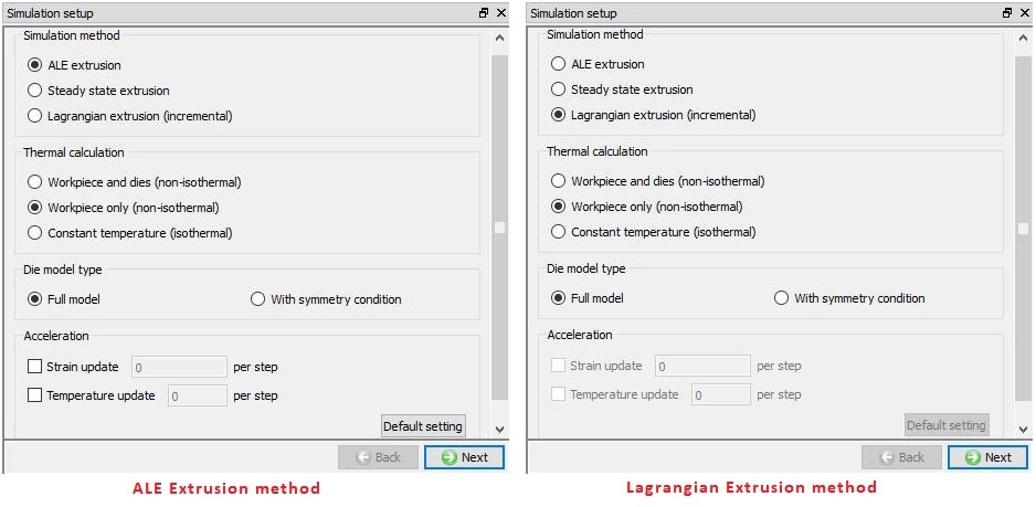
Simulation setup Page
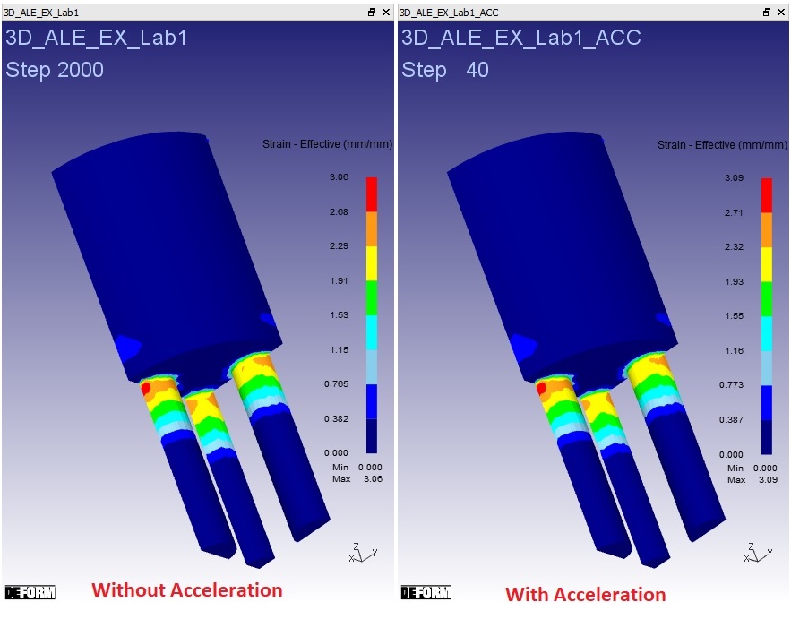
The effect of acceleration
Material List page
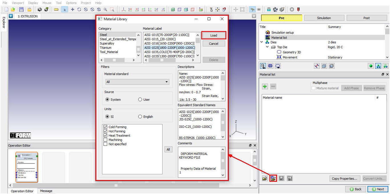
In material page, user can add materials to list from Load form Library option ![]() (As shown in Fig. 31.1.6.). If the desired material is not available in the list, then the user can load the material in object material page using Import Material data from a File
(As shown in Fig. 31.1.6.). If the desired material is not available in the list, then the user can load the material in object material page using Import Material data from a File ![]() . User can also create new material if the material is not available in DEFORM library using
. User can also create new material if the material is not available in DEFORM library using ![]() . User can delete the material from list using
. User can delete the material from list using ![]() or edit the material data using
or edit the material data using![]() . Modified / newly defined Material can be saved using
. Modified / newly defined Material can be saved using ![]() and
and ![]() .
.
Material list Page
Defining Extrusion Dies
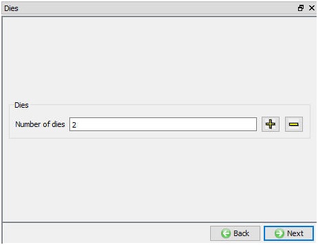
User can add dies by clicking on the ![]() button next to “Number of dies” field and if user wants to remove the dies then we must click on
button next to “Number of dies” field and if user wants to remove the dies then we must click on ![]() button as shown in the Fig. 31.1.7.
button as shown in the Fig. 31.1.7.
Dies Page
Die Object Page
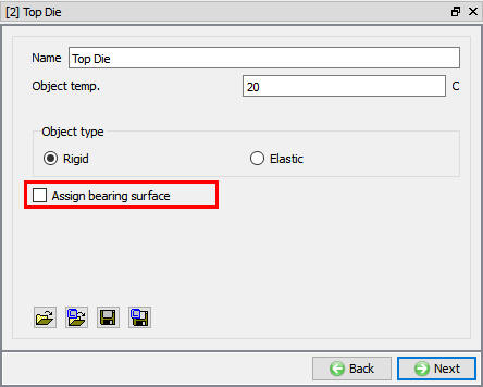
The user can define the Name, object temp. and object type (see Fig. 31.1.8.). The Rigid object type is selected by default, User can import objects from other databases or key files using ![]() ,
, ![]() options or save the object data using
options or save the object data using ![]() ,
,![]() options. User can observe “Assign bearing surface ” check box if the simulation type selected is ALE or Steady-state, user can check this check box for the die that has opening to define and modify the bearing surface.
options. User can observe “Assign bearing surface ” check box if the simulation type selected is ALE or Steady-state, user can check this check box for the die that has opening to define and modify the bearing surface.
Die object Page
###
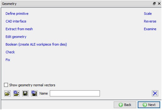
Geometry 3D
We can create the geometry using the “Define primitive” or we can import the geometry from a file using ![]() ,
, ![]() options. User can save the geometry data using
options. User can save the geometry data using ![]() ,
,![]() options.. For more information on other Geometry options please refer 3D Geometry. (See Fig. 31.1.9.)
options.. For more information on other Geometry options please refer 3D Geometry. (See Fig. 31.1.9.)
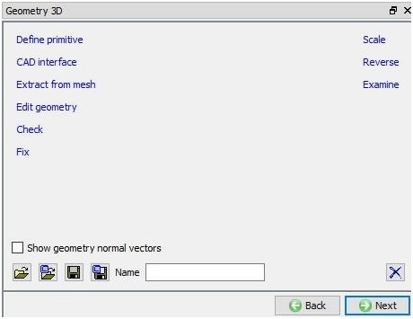
Die Geometry Page
Symmetry
The symmetry page is available only when we select the die model with symmetry condition in the simulation setup page.In this page, we can select the symmetry surface on the dies and workpiece using picking options.After selecting the symmetry surface click on ![]() button as shown in the Fig. 31.1.10. If user wants to delete any one defined symmetry surface data, select the respective surface data and click on
button as shown in the Fig. 31.1.10. If user wants to delete any one defined symmetry surface data, select the respective surface data and click on ![]() button. If user wants to delete all the symmetry data click on
button. If user wants to delete all the symmetry data click on ![]() button.
button.
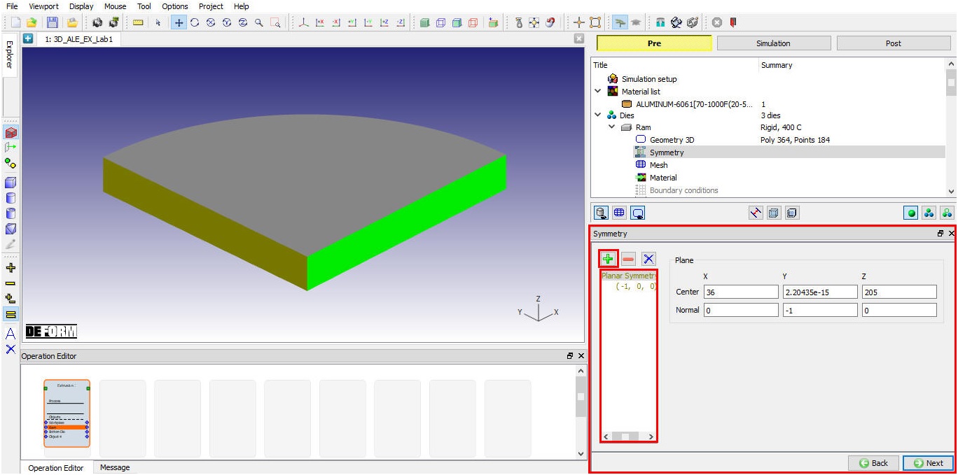
Symmetry Page
Dies Mesh Page
We can generate the mesh for dies by specifying the number of elements in guided mode as shown in the Fig. 31.1.11. Advanced options to control 3D mesh generation can be accessed using expert mode toggle button from tool bar.
For more information on the advanced mesh options from expert mode refer to the3D Mesh Setting.
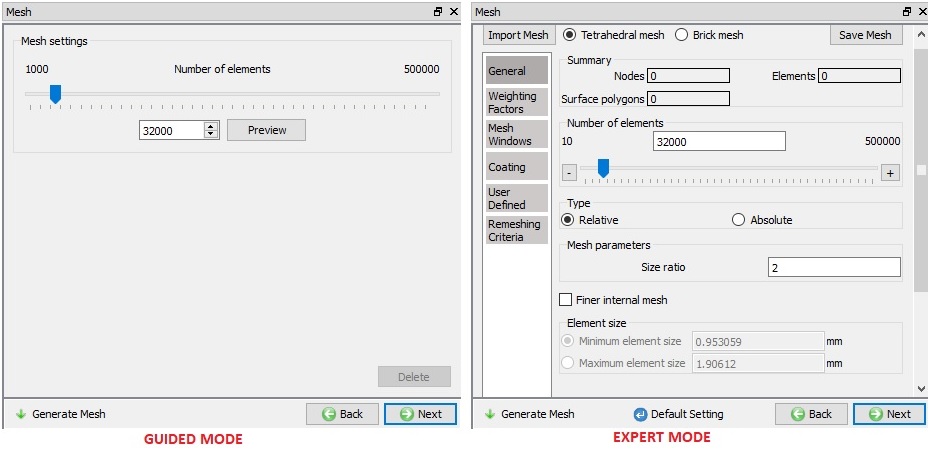
Dies Mesh Page
###
Material Selection
In material page, all the materials added to material list are displayed (As shown in Fig. 31.1.12.). User can select the required material to assign it to respective object. If the desired material is not available in the list, then the user can load the material in object material page using Import Material data from a File ![]() or Using Load form Library option
or Using Load form Library option ![]() . User can also create new material if the material is not available in DEFORM library using
. User can also create new material if the material is not available in DEFORM library using ![]() . User can delete the material from list using
. User can delete the material from list using ![]() or edit the material data using
or edit the material data using ![]() . Modified / newly defined Material can be saved using
. Modified / newly defined Material can be saved using ![]() ,
, ![]() .
.
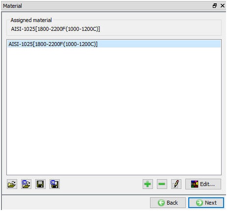
Assigning the material
###
BCC Page
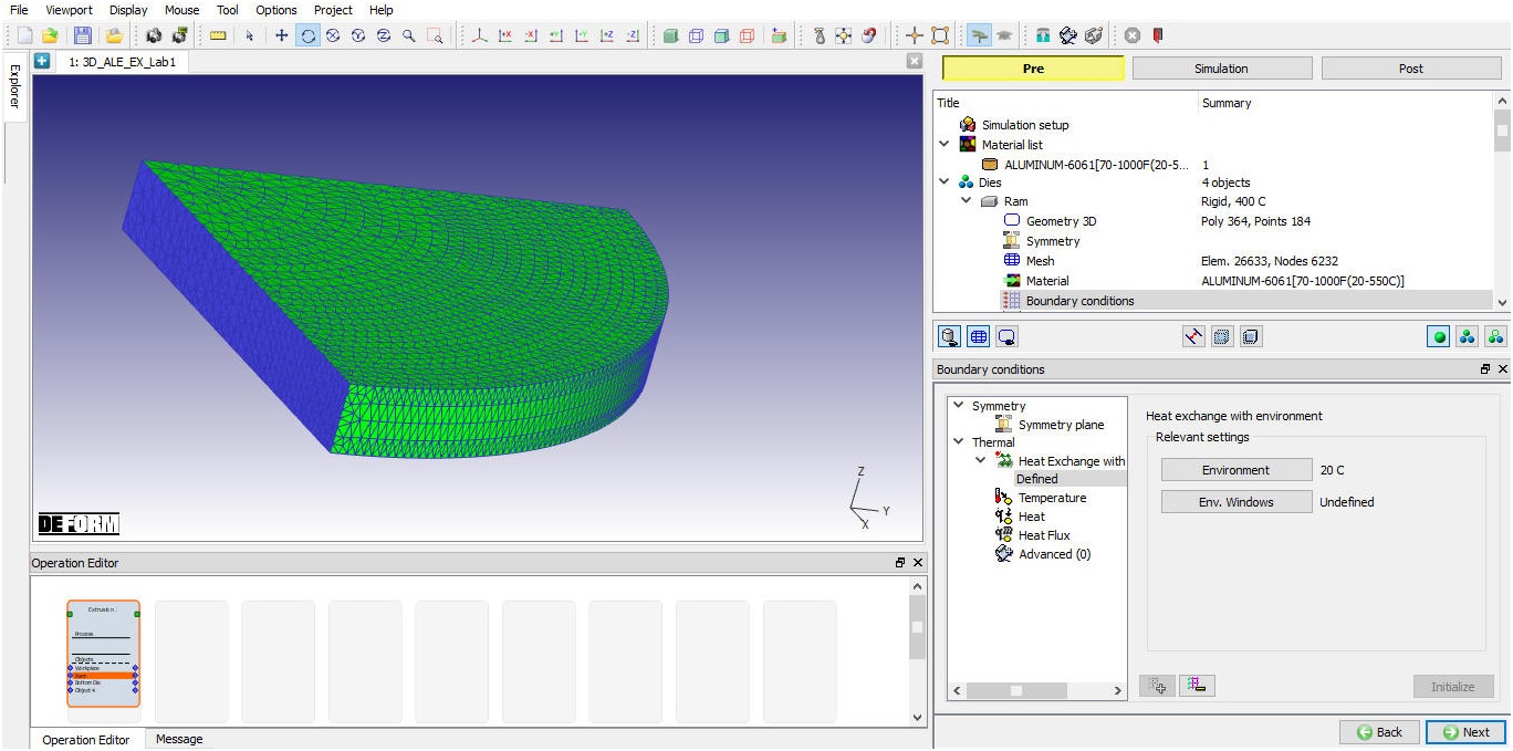
In Boundary conditions page, user can assign various boundary constraints to an object. Boundary conditions specify how the boundary of an object interacts with other objects and with the environment. Commonly used boundary conditions are heat exchange with the environment for simulations involving heat transfer and symmetry BCC for symmetry model. The Heat Exchange with environment BCC is added by default after mesh is generated as shown in the Fig. 31.1.13.
BCC Page
###
Movement
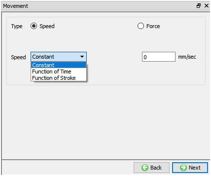
If the die is ram then user can define the movement for die based on Speed or Force as constant, Function of time or Function of Stroke as shown in the Fig. 31.1.14.
Die Movement Page
###
Bearing surface page (For ALE and Steady state extrusion)
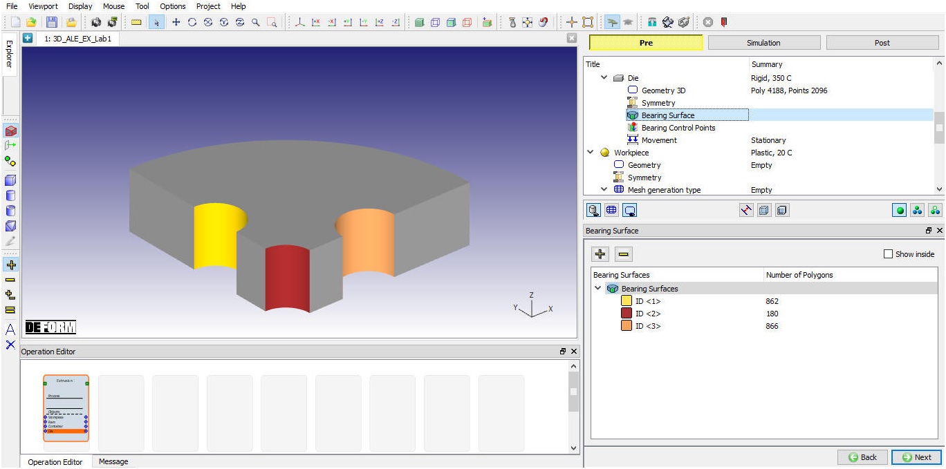
InBearing Surface page, we will define bearing surfaces and add them to the bearing surface list. To define the bearing surface, user can select all the patches related to the bearing surface and click ![]() button. A highlighted bearing surface with ID <1> **will be added to the list when we define the first bearing surface. Then user can go ahead and define other bearing surfaces similarly as shown in Fig. 31.1.15. Each of the bearing surface will be assigned unique ID and highlighted with different colors respectively in the die geometry display.
button. A highlighted bearing surface with ID <1> **will be added to the list when we define the first bearing surface. Then user can go ahead and define other bearing surfaces similarly as shown in Fig. 31.1.15. Each of the bearing surface will be assigned unique ID and highlighted with different colors respectively in the die geometry display.
**Show inside check box is used to see the inside geometry to select the bearing surface.
Added Bearing surfaces list
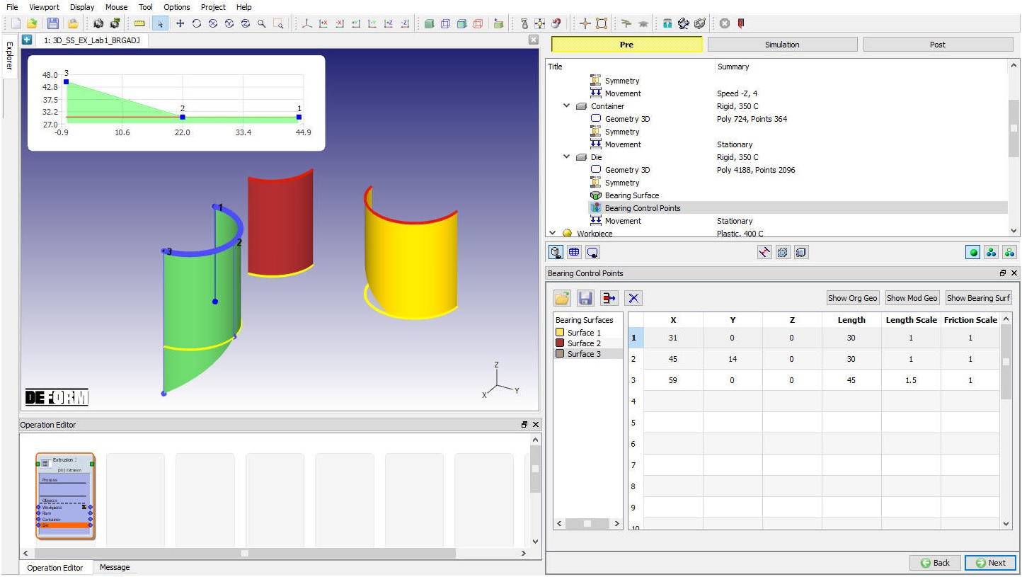
Bearing Control Points (For ALE and Steady state extrusion)
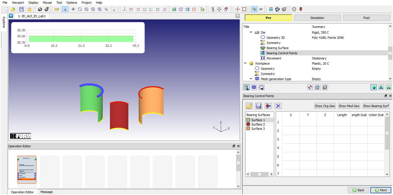
In extrusion, bending, wrap and twist of profiles are mainly caused by the unbalance material flowing. So, we can use bearing length adjustment to reduce the bending of surround profiles by defining the Bearing control points (see Fig. 31.1.16.). After defining the bearing surface user can define bearing control points along the entry edge of the bearing surface. The user can save the bearing control points in a file using ![]() button and can also import the saved bearing control points from a file using
button and can also import the saved bearing control points from a file using ![]() button. We can see the bearing shape and bearing length for surfaces are changed after defining the control points as shown in the Fig. 31.1.17.
button. We can see the bearing shape and bearing length for surfaces are changed after defining the control points as shown in the Fig. 31.1.17.
User can delete the selected bearing control point using ![]() button.
button.
User can delete all the control points of a bearing surface using ![]() button.
button.
Show Original Geometry![]() : Using this option we can see the original die geometry without applying modified bearing length values.
: Using this option we can see the original die geometry without applying modified bearing length values.
Show modified Geometry ![]() : Using this option we can see the modified die geometry after applying modified bearing length values, see Fig. 31.1.18.
: Using this option we can see the modified die geometry after applying modified bearing length values, see Fig. 31.1.18.
Show Bearing Surface ![]() : Using this option we can see only the defined bearing surfaces.
: Using this option we can see only the defined bearing surfaces.
Bearing control points page
Control points setting of bearing surface
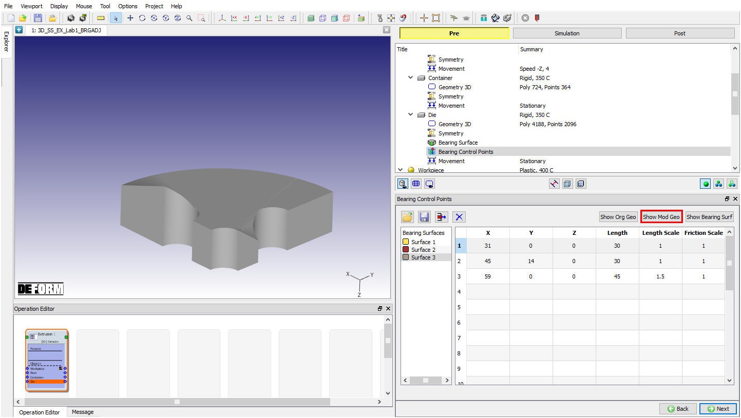
Modified die geometry after bearing length adjustment
For more information please refer to the steady state extrusion lab.
Defining Extrusion Billet
The user can select the Name and object temp. The object type will be plastic by default as shown in the Fig. 31.1.19.
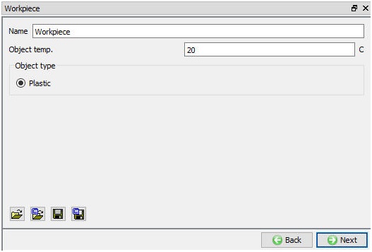
Workpiece object page
Workpiece Geometry Page
The workpiece geometry is created using the “Define primitive” or we can import the geometry using the import options. In case of ALE type simulation setup, workpiece geometry can be created using Boolean label after creating the dies geometry. For more information on other options in “Geometry” page, please refer 12.3. 3D Geometry Data Defining.
Workpiece Geometry page
###
Workpiece Mesh Generation Type
In Extrusion template user can generate regular tetrahedral mesh for workpiece using “Regular meshing” method or special mesh using “Mesh extruding utility”, see Fig. 31.1.21.
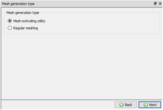
Mesh generation types
- Workpiece Mesh extruding utility
Mesh Extruding utility is a special type of meshing used in Extrusion operation to generate mesh within less time. In this meshing method the workpiece is categorised into 3 Regions,
-
Container Region – This region consists of material within container that does not have severe deformation.
-
Deforming Region - This is the region closer to die opening where we can observe severe deformation of material takes place. This region covers die opening and partly entry and exit of the material through die opening.
-
Extrudate Region – This region covers the material that has already passed through die opening and not much deformation would be occurring.
The zones are automatically identified by the system based on the geometry of the die. However, user can adjust the zones by dragging the respective zone boundaries in the representative image in mesh extruding utility window, see Fig. 31.1.22. or use window control points in display area. User can control the mesh transition using the settings in “Mesh Extruding Utility” window.
In this method, tetrahedral mesh is created in the deforming region and then the tetrahedral mesh is extruded into container region and extrudate region, see Fig. 31.1.23. User can create a multiple zones in each region and define size ratio/ number of layers for each zone to control the mesh transition. In deforming region mesh can be generated using,
-
Relative : In this method user can define the # of elements to generate the relative mesh and define size ratio in each zone to control the mesh transition.
-
Absolute : In this method user can define the Min. element size value and define element size in each zone to control the mesh transition.
Preview : When user clicks on “Preview ” action then tet mesh is generated for deforming region and displayed.
Generate : User can click on “Generate ” action item to generate mesh.
Default Setting ![]() : When user clicks on this button then zones and its values are set back to the default values.
: When user clicks on this button then zones and its values are set back to the default values.
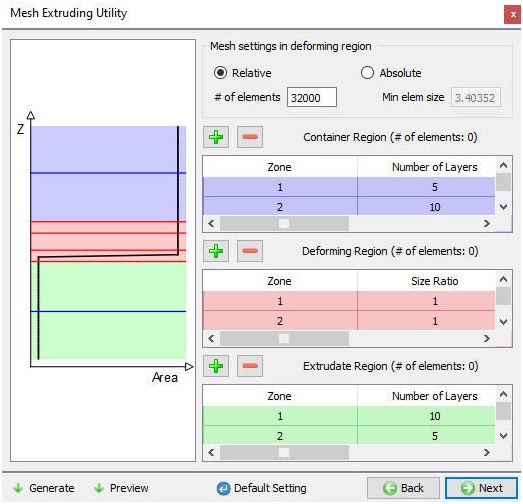
Mesh extruding utility page
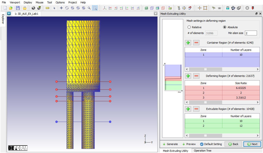
Mesh Generated using the mesh extruding utility options
- Workpiece Regular meshing
In the regular mesh setting user can control mesh by defining advanced settings like weighting factors, mesh windows, size ratioand remeshing criteria. User can click on “![]() ” to generate mesh, mesh generated using regular meshing looks like as shown in the Fig. 31.1.24.
” to generate mesh, mesh generated using regular meshing looks like as shown in the Fig. 31.1.24.
For more information on mesh settings in regular meshing refer Expert mode mesh settings in 13.2.2. Expert mode 3D mesh generation
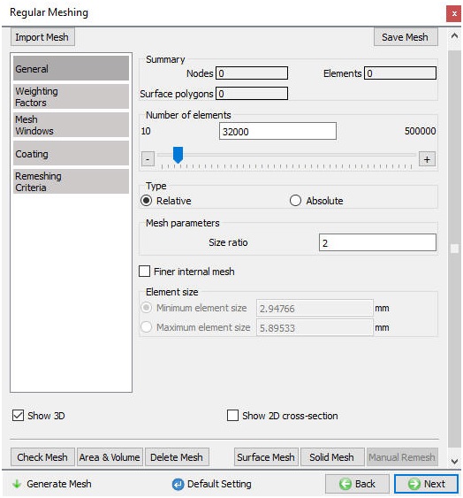
Regular meshing page
###
Workpiece BCC Page
In Boundary conditions page, user can assign various boundary constraints to an object. Boundary conditions specify how the boundary of an object interacts with other objects and with the environment. The system automatically assigns the symmetry plane BCC to the symmetry model workpiece after mesh generation (see Fig. 31.1.25.).
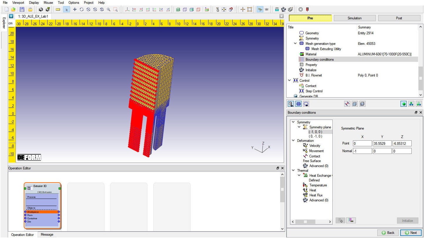
Symmetry BCC of the Workpiece
BCC for ALE and Steady-state extrusion simulation methods
In case of ALE and Steady-state simulation methods user must define the Free Surface. Free surface is the surface at exit end of the extrudate. In the Boundary conditions dialog, click Free Surface in the tree,select the bottom surface and then Click ![]() to add the Free surface boundary condition (see Fig. 31.1.26.).
to add the Free surface boundary condition (see Fig. 31.1.26.).
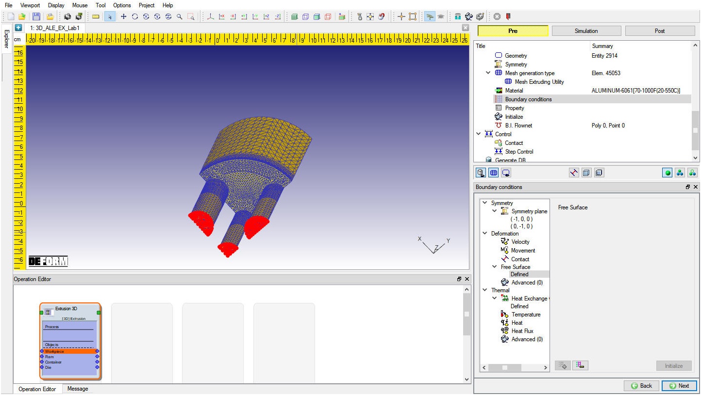
Free Surface BCC of the Workpiece
Property
Miscellaneous object parameters, which affect either thermo-mechanical behaviour of the object or numerical solution behaviour are specified in the Object-Properties window. (See Fig. 31.1.27.). Volume compensation in one of the important parameters to be set in Lagrangian type of extrusion simulation, it can be activated by selecting one of the options under “Target Volume” and calculating current object volume using ![]() button. For more information about options in “Property ” page, please refer 16. Object properties.
button. For more information about options in “Property ” page, please refer 16. Object properties.
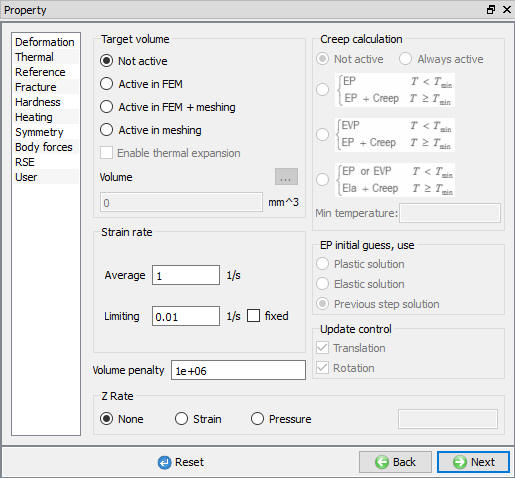
Property page
Initialize
In Initialize window, few state variables that are commonly used such as temperature, strain, stress, damage, velocity, displacement, density and microstructure grain size and particle size are made available for initialization.
User can initialize the values for these state variables by defining in the field next to it and clicking on ![]() button. Fig. 31.1.28. shows various state variables that are available in “Initialize” window. Depending on the type of state variable, user can also initialize them from Node and Element data windows. For more information on how to initialize state variables in Node and Element windows, please refer Object node variables and Object element variables.
button. Fig. 31.1.28. shows various state variables that are available in “Initialize” window. Depending on the type of state variable, user can also initialize them from Node and Element data windows. For more information on how to initialize state variables in Node and Element windows, please refer Object node variables and Object element variables.
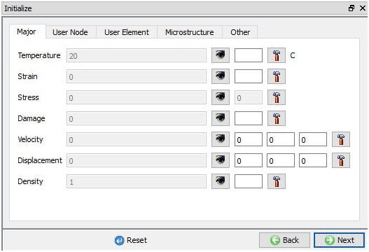
Initialize page
B.I. Flownet
In a DB with large number of steps, plotting a Flownet will take lot of time, user can overcome this issue by using Built in Flownet. When user uses Built in Flownet, the Flownet is plotted as the problem is simulated. (See Fig. 31.1.29.)
For more information on defining Built in Flownet,please refer 13.2.9. Built in Flownet

Built-in Flownet page
Controls
User can position the objects using ![]() button. Various positioning options are available to position the objects as shown in Fig. 31.1.30., for more information on these options please refer 19. Object positioning.
button. Various positioning options are available to position the objects as shown in Fig. 31.1.30., for more information on these options please refer 19. Object positioning.
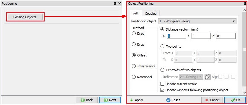
Object Positioning Controls
Contact
In extrusion operation template a special contact method has been implemented to generate complete contact over billet in case of ALE and Steady-state simulation methods to reduce the simulation time to achieve steady-state. When the user visits the contact page, we will get the “Full Contact Generation” pop-up as shown in the Fig. 31.1.31. In full contact generation is used, it will automatically calculate the contact tolerance with the neighbouring objects and then generates contact.
In case of Lagrangian type of simulation method user can estimate tolerance using ![]() and then generate contacts.
and then generate contacts.
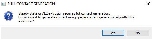
Full Contact Generation pop-up
System : When this radio button is selected, system assigns default inter-object relationships. Also, user can add the lubricants if necessary, by selecting Add New from pull down menu and clicking on “Edit” button or user can load the required lubricants from the library for the simulation.
User : By default, user radio button will be selected for Extrusion operation. User can add relationships by clicking on ![]() button as shown in Fig. 31.1.32. User can modify the value of each relation by selecting it and clicking on
button as shown in Fig. 31.1.32. User can modify the value of each relation by selecting it and clicking on ![]() button. User can use
button. User can use ![]() to assign same values to all relations. User can click on
to assign same values to all relations. User can click on ![]() to calculate contact tolerance. User can click on
to calculate contact tolerance. User can click on ![]() to generate contact relation between objects that have contact relations defined. User can turn on check box next to contact relation to define sticking contact.
to generate contact relation between objects that have contact relations defined. User can turn on check box next to contact relation to define sticking contact.
For more information on contact dialog, please refer 20.Inter-Object Relations.
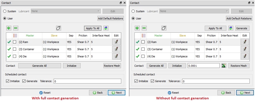
Contact Page
Step Controls
In step controls, user can define the number of steps, step increment and Time/Stroke per step to control the simulation steps as shown in the Fig. 31.1.33. Step controls that need to be defined are provided in guided mode while more advanced settings can be defined in Expert mode.
GUIDED MODE:
Number of steps:Number of steps to be simulated can be defined here. If the simulation stops earlier due to stopping criteria then, next operation starting step will be continuation from previous operation.
Step increment : The step increment (STPINC) to save in the database controls the number of steps that the system will save in the database. When a simulation runs, every step must be computed, but does not necessarily need to be saved in the database. Storing more steps will preserve more information about the process, consequently it will require more storage space.
Time per Step: If time per step is specified, the time interval per step will be used. The die displacement per step will be the time step times the die velocity.
Stroke per Step: If stroke per step is specified, the primary die will move by specified amount in each time step. The total movement of the primary die will be the displacement per step multiplied by the total number of steps.
Primary Die: The primary die (PDIE) is the object for which many stopping and stepping criteria are defined. For example, stopping distance based on primary die stroke. When the stroke of the object defined as the primary die reaches the value of primary die displacement, the simulation will be stopped even though more steps were specified. The Step by Stroke feature determines step size based on the movement of the primary die.
The primary die is usually assigned to the object most closely controlled by the machinery. For example, the die attached to the ram of a hydraulic press would be designated as the primary object.
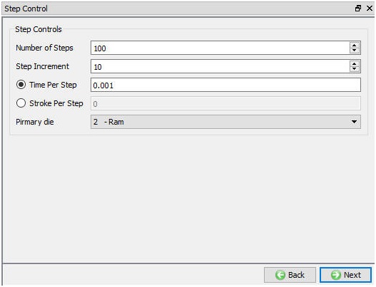
Step Controls in GUIDED Mode
###
EXPERT MODE
The user can define the step controls data using the expert mode simulation controls as shown in the Fig. 31.1.34. For more information and description about options in expert mode simulation controls, please refer 9. Simulation Controls.
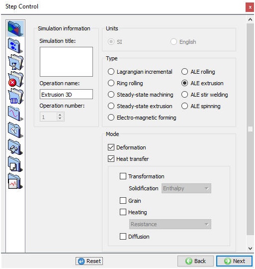
Step controls in EXPERT Mode
Generate DB
Check Data![]() **
**
It checks the Data. If Data is correct we can generate DB. But while checking Data if it gives any errors or warnings then it should be corrected before generating Database. Errors will not allow the database to be generated while warnings will allow the DB to be generated.
Generate Database![]()
By clicking on this button, it generated the Database for the setup.(See Fig. 31.1.35.)
Append Key file
Any information that is not defined in the wizard but still applicable to the process can be loaded as .key file. This option is also useful in the cases where only few values needs to be changed then those values can be defined as .key file and only .key file can be changed and simulation can be resubmitted.

Generate DB page
Related Topics: