2D Heat Treatment Wizard Lab1
1.1. Introduction
1.2. Starting a New problem
1.3. Process Settings
1.4. Material definition
1.5. Workpiece Object Type
1.5.1. Defining Workpiece Object Data
1.5.2. Import Geometry
1.5.3. Generate Mesh
1.5.4. Assigning Material
1.5.5. Generating Coating Mesh
1.5.6. Assigning Boundary conditions
1.5.7. Workpiece Phase levels initialization
1.6. Medium Definition
1.7. Scheduled Definition
1.8. Simulation controls
1.9. Generate Database
1.10. Starting the Simulation
1.11. Post processing
Introduction
The Heat Treatment Wizard is a convenient tool to set up complex multiple-operation heat treatment problem. This lab will demonstrate how to use this wizard to prepare a carburization-quench-tempering simulation of a steel part. This lab can also help users understand the capabilities of DEFORM-HT’s phase transformation calculation scheme.
Starting a New problem
On a Windows machine , go to the ![]() button select DEFORM-v1x.xxx (.xxx indicates version number E.g. v14.0.2) and select DEFORM GUI Main vxx.xx from the menu. The DEFORM GUI Main window will appear
button select DEFORM-v1x.xxx (.xxx indicates version number E.g. v14.0.2) and select DEFORM GUI Main vxx.xx from the menu. The DEFORM GUI Main window will appear
Create a new problem either by selecting File![]() **New Problem** or by clicking the New Problem
**New Problem** or by clicking the New Problem ![]() icon. The Problem Setup window will appear as shown in Fig. 2DHTWL1.1. Select “ Integrated Manufacturing Process “ radio button and units system as “SI “ using radio button. Define Problem Name as “QUENCH “ and make sure the “Show option dialog” check box is turned on (if we do not turn on the “Show option dialog ” check box, then we will not get the New Project dialog in MO UI). Then click on
icon. The Problem Setup window will appear as shown in Fig. 2DHTWL1.1. Select “ Integrated Manufacturing Process “ radio button and units system as “SI “ using radio button. Define Problem Name as “QUENCH “ and make sure the “Show option dialog” check box is turned on (if we do not turn on the “Show option dialog ” check box, then we will not get the New Project dialog in MO UI). Then click on ![]() button to open a new Problem using the Deform Integrated Manufacturing Process.
button to open a new Problem using the Deform Integrated Manufacturing Process.
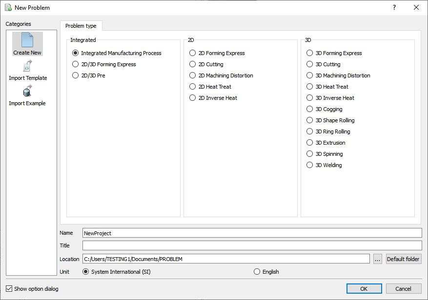
Problem type selection window
Multiple operation wizard will open with the New Project dialog as shown in Fig. 2DHTWL1.2., at this point user will be prompted to specify a project name (system will create a separate folder with this project name) and title. In this lab we will use ‘QUENCH ’ as the project name.
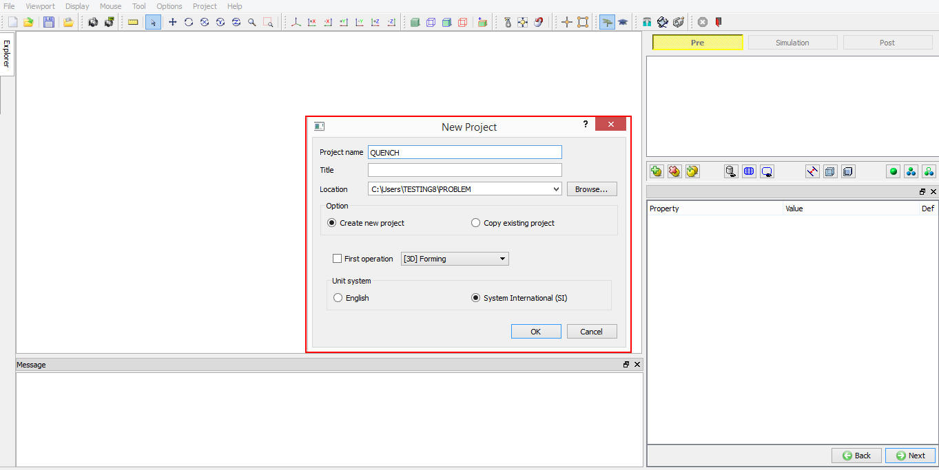
MO wizard New project
User can also change the Unit system (File menu selected unit system will be selected by default) and add HT operation by selecting it from First operation pull down list and turning on checkbox (See Fig. 2DHTWL1.3.). Using copy Existing project option, we can import previous saved projects as new project. Click on ![]() to continue to open the operation.
to continue to open the operation.
Multiple Operation wizard will open. Add 2D HT Wizard operation from the Explorer Operations list. Add the operation by clicking on ![]() button next to 2D HT Wizard or user can also add by drag and drop into the Operation Editor (See Fig. 2DHTWL1.3..).
button next to 2D HT Wizard or user can also add by drag and drop into the Operation Editor (See Fig. 2DHTWL1.3..).
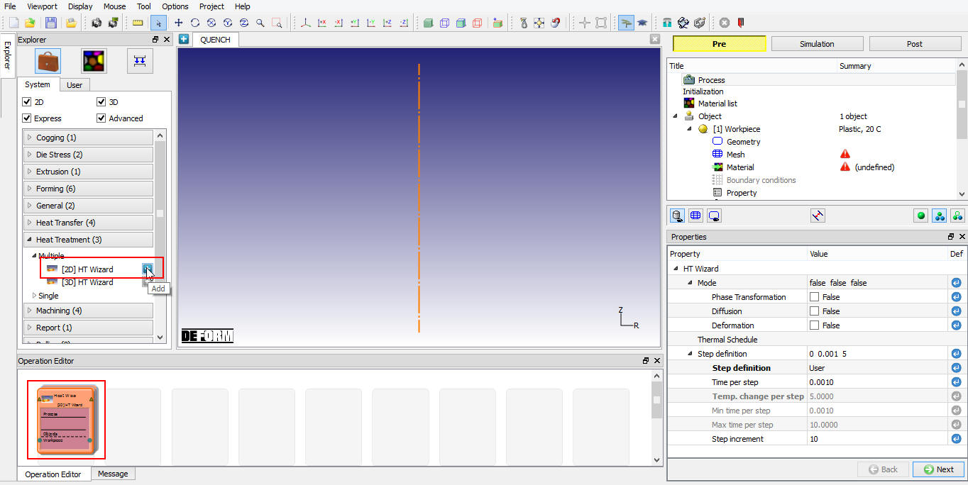
Adding 2D HT Wizard into Operation Editor
Process Settings
As the operation is added, Process settings page is opened as shown in Fig. 2DHTWL1.4. User can set the simulation mode based on the simulation requirement along with step definition controls.
Turn on “Deformation “ and “PhaseTransformation “ as we would like to predict residual stresses and phase transformation calculations during the process. Step definition will be defined in Simulation controls page. Click ![]() (See Fig. 2DHTWL1.4.).
(See Fig. 2DHTWL1.4.).
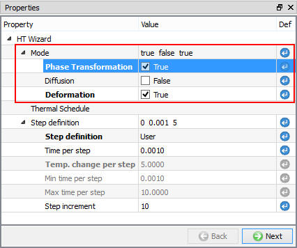
Defining Process settings in 2D HT Wizard
Initialization page will open, we can observe that Phase transformation and Deformation check boxes are turned on (See Fig. 2DHTWL1.5.), we will leave the settings in Initialization page as it is and click ![]() .
.
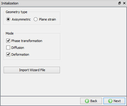
Initialization Setup window
Material definition
In Material window, load the material (JIS-S45C (Heat Treatment)) from DEFORM Material library, from Steel category using ![]() (Load material data from library) option. This can be done as shown in Fig. 2DHTWL1.6. by clicking
(Load material data from library) option. This can be done as shown in Fig. 2DHTWL1.6. by clicking ![]() button. Material can also be load from Materials list in Explorer. Then click
button. Material can also be load from Materials list in Explorer. Then click ![]() unitl Workpiece page.
unitl Workpiece page.
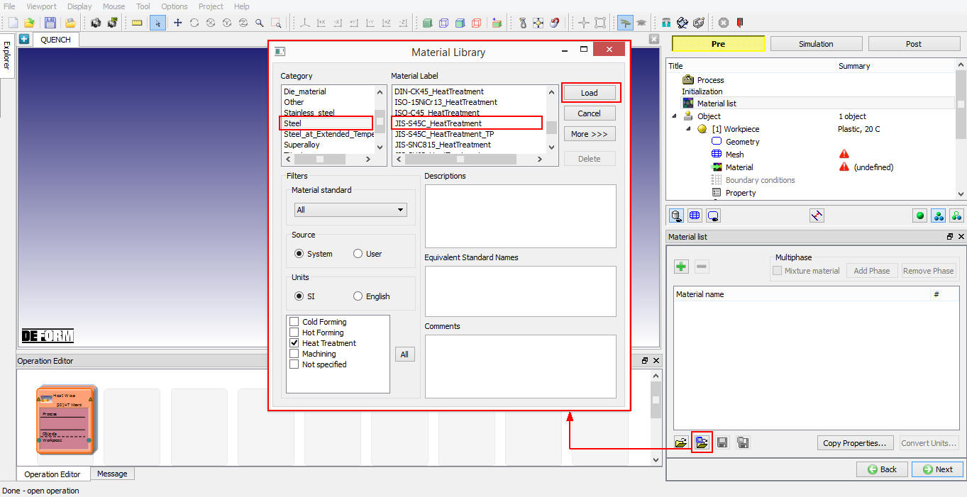
Importing Material page
Defining Workpiece
Defining Workpiece Object Data
In Workpiece page, change the object type to Elasto-plastic type, as we need to predict residual stresses (See Fig. 2DHTWL1.7.). Set object temperature as 900 °C. Click ![]() .
.
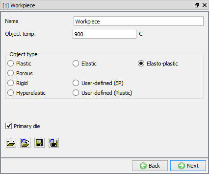
Workpiece object definition
Import Geometry
In Geometry page, click on ![]() (import geometry from library) option and import the QUENCH_PART.IGS file from installation path \SFTC\DEFORM\v_\2d\LABS as shown in Fig. 2DHTWL1.8. Use
(import geometry from library) option and import the QUENCH_PART.IGS file from installation path \SFTC\DEFORM\v_\2d\LABS as shown in Fig. 2DHTWL1.8. Use ![]() action label to check the Geometry. A perfect geometry should display message as shown in Fig. 2DHTWL1.9. Click
action label to check the Geometry. A perfect geometry should display message as shown in Fig. 2DHTWL1.9. Click ![]() .
.
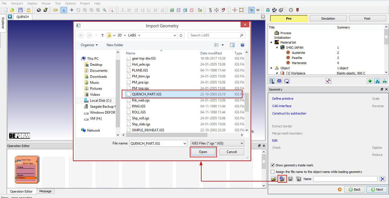
Importing Geometry for Workpiece
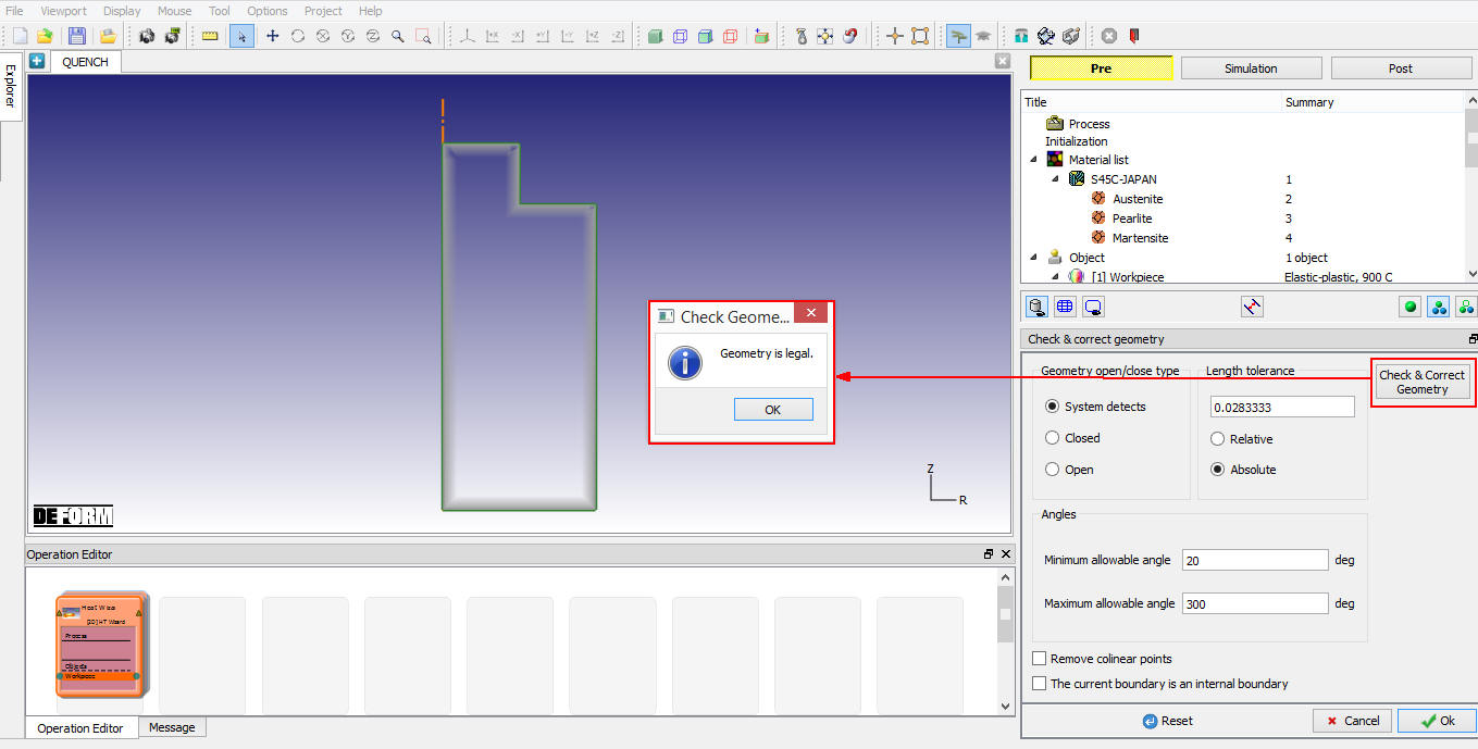
Output of imported geometry checking
Generate Mesh
In Mesh page, enterTarget number of elements as 500 and click on ![]() button. After completion of generating mesh, click on
button. After completion of generating mesh, click on ![]() button to assign material for workpiece.
button to assign material for workpiece.

Mesh settings and mesh generated
Assigning Material
Select and assign S45C-JAPAN Material as shown in Fig. 2DHTWL1.11. Click ![]() to generate coating mesh.
to generate coating mesh.
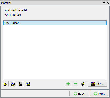
Assigning Material to workpiece
Generating Coating Mesh
Switch to expert mode by click on ![]() . We will be adding coating layers to obtain better information about the phase transformations on surfaces. Select Coating tab and add 2 layers by clicking on
. We will be adding coating layers to obtain better information about the phase transformations on surfaces. Select Coating tab and add 2 layers by clicking on ![]() button. Set 500 and 1000 for thickness of layer 1 and 2 respectively as shown in Fig. 2DHTWL1.12., select same material S45C-JAPAN and click on
button. Set 500 and 1000 for thickness of layer 1 and 2 respectively as shown in Fig. 2DHTWL1.12., select same material S45C-JAPAN and click on ![]() button. Click on
button. Click on ![]() to change to guided mode. Click
to change to guided mode. Click ![]() until boundary conditions page.
until boundary conditions page.
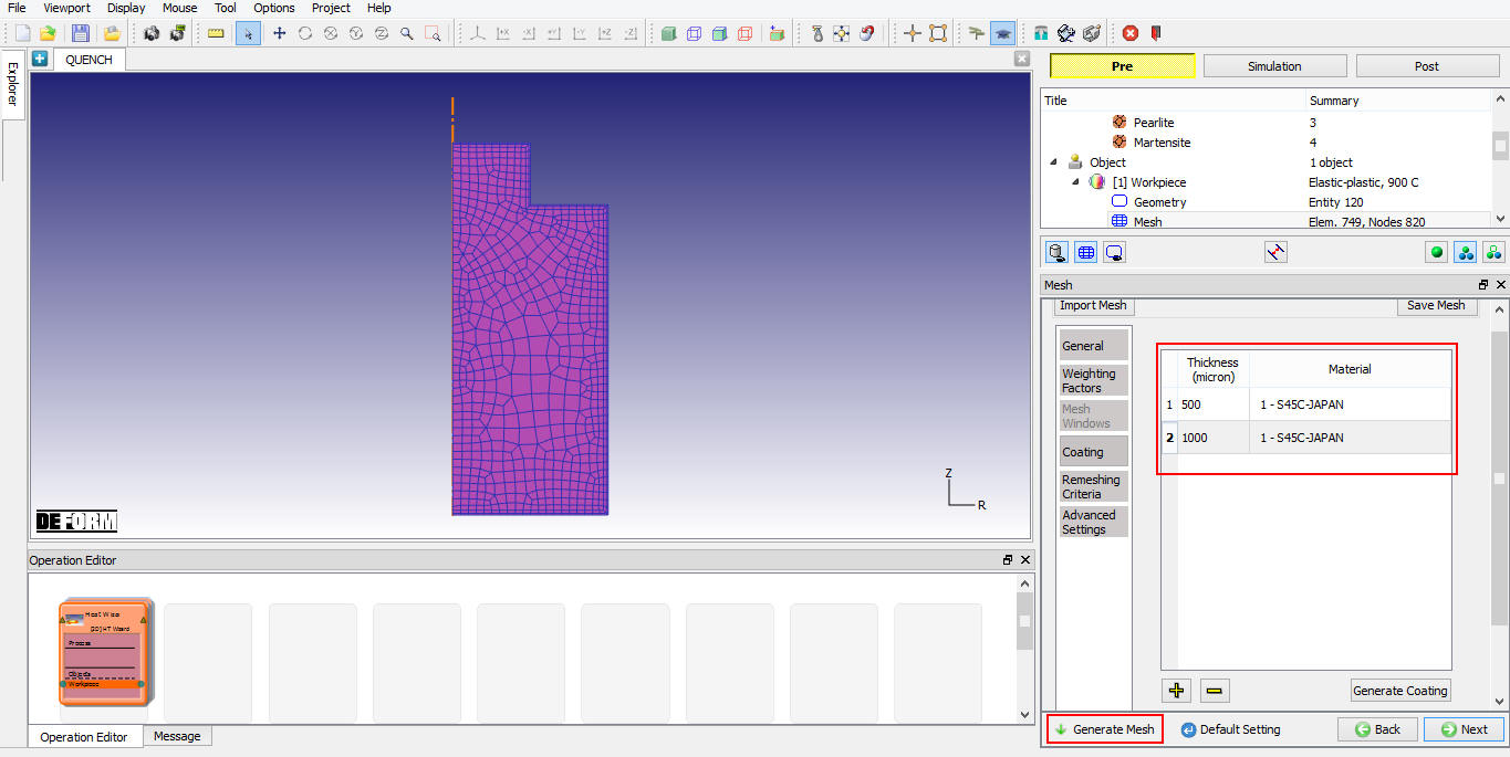
Coating mesh settings used in Workpiece mesh generation
Assigning Boundary conditions
-
Select X direction and define velocity as 0, pick nodes along axis as shown in Fig. 2DHTWL1.13. to constrain nodal velocity in X direction, as this is an axi-symmetric set up.
-
Select Y direction and define velocity as 0, pick nodes along bottom surface of the workpiece as shown in Fig. 2DHTWL1.13. to constrain nodal velocity in Y direction of workpiece during quench.
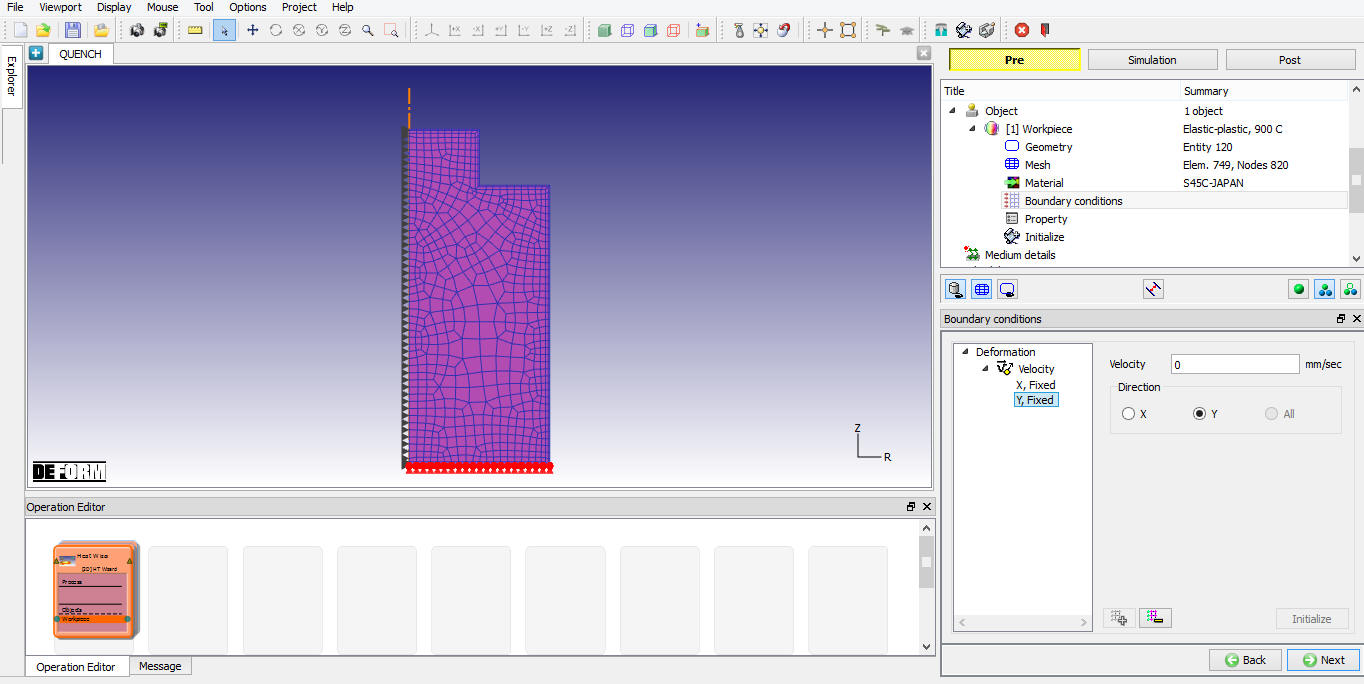
Assigning Velocity BCC
Workpiece Phase levels initialization
Since we need to calculate phase transformation, we need to initialize initial level of each phase, keep note that sum of all phases at each element should be equal to 1. Since the object temp is 900°C and the material is steel, the material would have changed to Austenite phase completely, we will initialize entire workpiece to Austenite phase. To do so, click on object element data ![]() and select Phase transformation tab under Microstructure. Initialize Austenite as 1 and zero for the rest by selecting phase and using
and select Phase transformation tab under Microstructure. Initialize Austenite as 1 and zero for the rest by selecting phase and using ![]() (See Fig. 2DHTWL1.14.). In Initialize Element Data window assign value using Range option by defining 1 as value as shown in Fig. 2DHTWL1.15. and then click on
(See Fig. 2DHTWL1.14.). In Initialize Element Data window assign value using Range option by defining 1 as value as shown in Fig. 2DHTWL1.15. and then click on ![]() button. Click on
button. Click on ![]() button to close the Initialize Element Data window and click
button to close the Initialize Element Data window and click ![]() to close Element data dialog. Click
to close Element data dialog. Click ![]() to define the medium details.
to define the medium details.
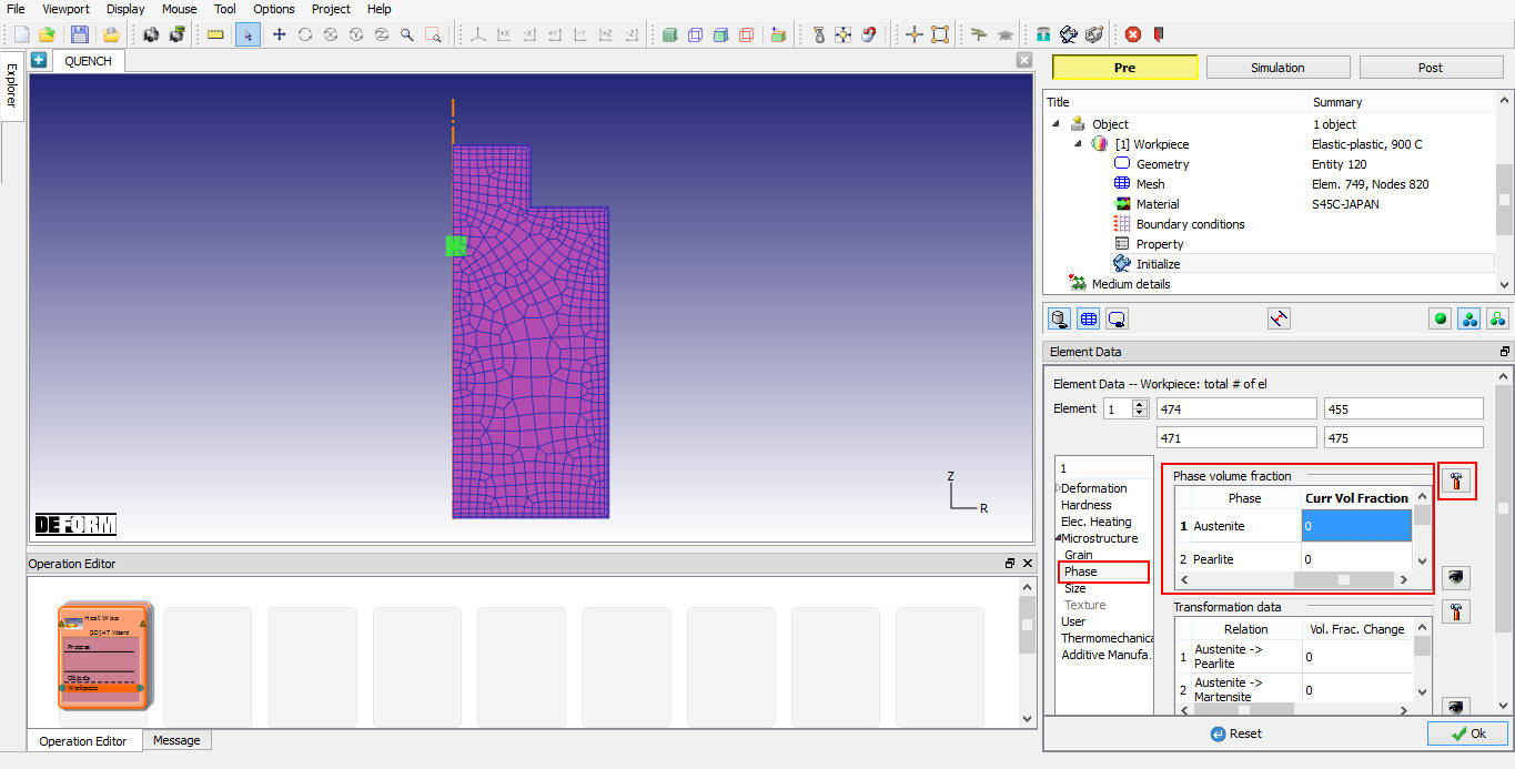
Phase level initialization in object Element Data
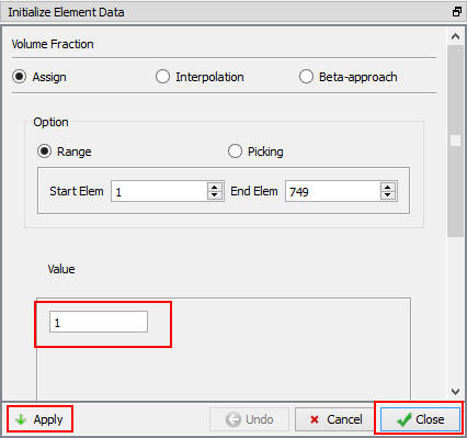
Element Data initialization window
Medium Definition
The simulation consists of quenching, we need to define required medium for this operation, in this case we require water and air. In page “Medium details”, you will define various media and heat transfer zones associated with them as shown in Fig. 2DHTWL1.16.
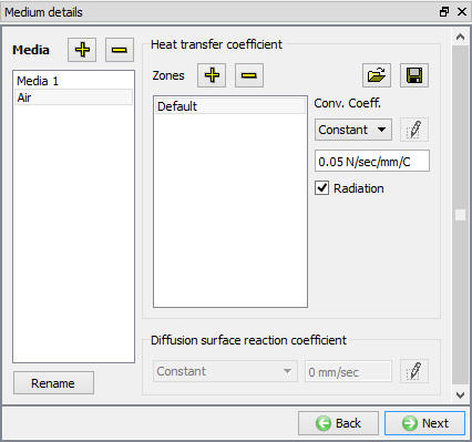
Medium Details window
-
Rename the first medium to “Air” and set the “Default” Heat transfer coefficient (HTC) and convection coefficient to constant 0.05 as shown in Fig. 2DHTWL1.16.
-
Add a media “Water”. For “Default” HTC, load convection coefficient data from file “WATER_HTC1_si.DAT”.
-
Add one more heat transfer zone under media “Water”. Click on the object boundary to specify the start and end points of the zone. The zone is assigned to the bottom of the workpiece as shown in Fig. 2DHTWL1.17. For Zone #1 HTC, load convection coefficient from file “ WATER_HTC2_si. DAT” and click on define function to observe the function data as shown in Fig. 2DHTWL1.18. Click
 to define the schedule page.
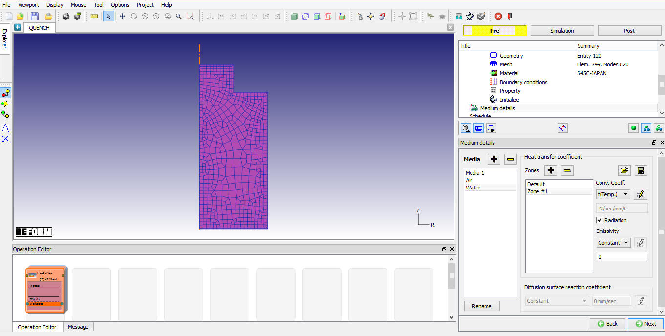
Medium detail window showing zone allocation
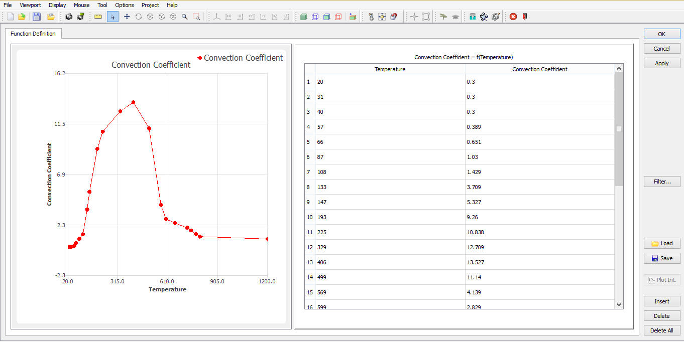
Function definition window
Scheduled Definition
In “Schedule” page, input a five-stage quench schedule as shown in Fig. 2DHTWL1.19. by clicking on ‘Add’ button. A procedure like this is sometimes referred as “Intensive Quenching”, which is designed to create a very thin “crust” of Martensite on the part. Such a process can achieve high surface hardness with relative low part distortion.
1) 20 seconds(20s) cooling in the air at 20C
2) 10 seconds(10s) cooling in the water at 70C
3) 60 seconds(60s) cooling in the air at 20C
4) 5 seconds(10s) cooling in the water at 70C
5) 20 Minutes(1200 s) cooling in the air at 20C
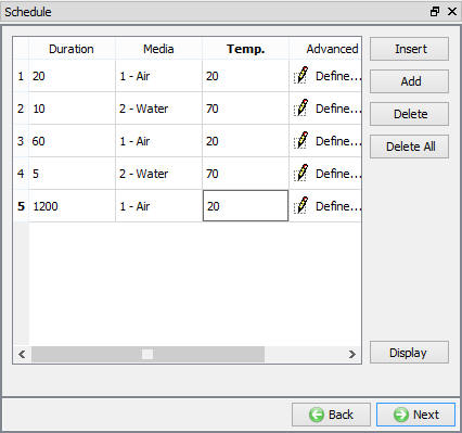
Heat Treatment Schedule window
The settings for each stage can be set or modified using ![]() button in advanced column. Click
button in advanced column. Click ![]() until Simulation controls page.
until Simulation controls page.
Simulation controls
In “Step Definition”, select Auto radio button and change “Temp. Change per step” to 5°C and keep other default settings. Click ![]() to DB generation page. (See Fig. 2DHTWL1.20.)
to DB generation page. (See Fig. 2DHTWL1.20.)
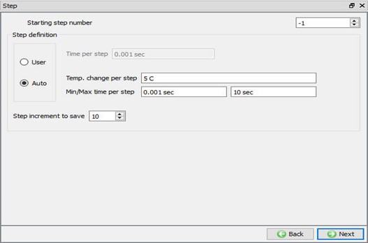
Simulation controls window
Generate Database
Click on ![]() action label to check the problem. Generate a database by clicking
action label to check the problem. Generate a database by clicking ![]() action label (see Fig. 2DHTWL1.21.). When the program is done writing the database, switch to
action label (see Fig. 2DHTWL1.21.). When the program is done writing the database, switch to ![]() tab to run simulation.
tab to run simulation.
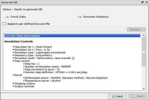
Generate Database Window
Starting the Simulation
Click on the ![]() action label to open the Run Options dialog as shown in Fig. 2DHTWL1.22. Use the default Continue Run option to select “Continue from the last step ” (from step -1) option and then select the Simulation mode as Interactive and click on
action label to open the Run Options dialog as shown in Fig. 2DHTWL1.22. Use the default Continue Run option to select “Continue from the last step ” (from step -1) option and then select the Simulation mode as Interactive and click on ![]() button to run the simulation. As we click on the
button to run the simulation. As we click on the ![]() button simulation starts.
button simulation starts.
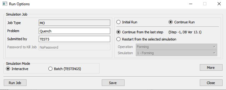
Run simulation window
The progress of the simulation can be monitored as it is running by looking at the Simulation Message and process monitor in Simulation mode. Click the Simulation Message tab to view the Message file. If ![]() option is checked, which is the default setting, the Message file will refresh every couple of seconds.
option is checked, which is the default setting, the Message file will refresh every couple of seconds.
The Message file provides information about which simulation step the simulation is currently on and gives information dealing with how well the simulation is running.
When the simulation has finished, the message will be added to the end of the Message file. (See Fig. 2DHTWL1.23.).
Each stage defined will be executed as individual operation and user need to wait until all the stages simulation is completed.
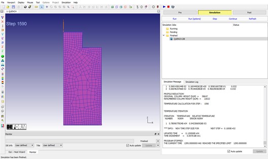
Simulation Message tab
Post processing
When the simulation has finished, click on ![]() . In Step Browser click on
. In Step Browser click on ![]() button to view all steps. Plot Temperature state variable and observe the temperature distribution at different stages of quenching operation (See Fig. 2DHTWL1.24.). Also plot the volume fraction of each phases at the end of the Quenching process using Volume fraction state variable under microstructure. (See Fig. 2DHTWL1.25.).
button to view all steps. Plot Temperature state variable and observe the temperature distribution at different stages of quenching operation (See Fig. 2DHTWL1.24.). Also plot the volume fraction of each phases at the end of the Quenching process using Volume fraction state variable under microstructure. (See Fig. 2DHTWL1.25.).
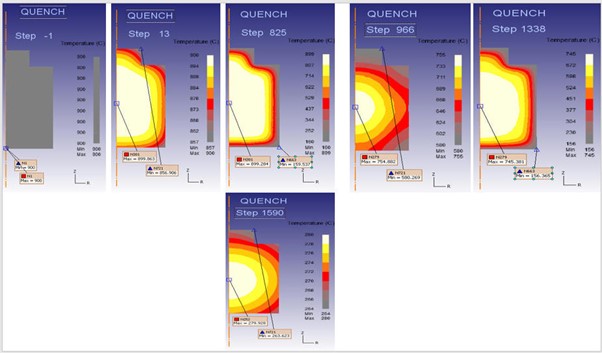
Temperature distribution at different stages of quenching operation.
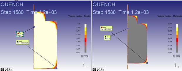
Volume fraction of each phases at the end of the Quenching process of quenching operation.