3D Cutting Lab1
1.1. Summary
1.2. Starting the 3D machining wizard
1.3. Define Machining Process data
1.4. Defining Insert geometry
1.5. Defining Tool Holder
1.6. Assigning Insert material
1.7. Generating insert mesh
1.8. Insert Boundary Conditions
1.9. Workpiece Geometry
1.10. Assigning Workpiece Material
1.11. Generating Mesh for Workpiece
1.12. Workpiece Boundary Condition page
1.13. Tool Positioning
1.14. Tool Wear Setting
1.15. Contact page
1.16. Step Control page
1.17. Generate Database
1.18. Running Simulation
1.19. Post Processing
Summary
This document details the current modeling capabilities available in DEFORM system to simulate 3D metal cutting environment in turning process. The system can be used to model the industrial turning process, without any assumptions that are associated with orthogonal cutting conditions. These modeling procedures enable the engineer to study the process response for any change in process conditions. Cutting forces, cutting temperatures, chip shape, tool wear and tool life computations can be performed using this system. The engineer can study the effect of process parameters like, cutting speed, feed rate and depth of cut on the process response. DEFORM® supports a special purpose template that simplifies the model definition and uses the same engineering language of process engineer. For turning applications, the rotating work piece, insert and their relation to the analysis domain are shown in Fig. 3DTL1.1. Typical analysis model generated using the current system is shown in Fig. 3DTL1.2. The main data requirements to model the machining process are material flow stress data for the work piece material and geometric data for the insert. The material flow stress data should cover the strain rate, strain and temperature range for metal cutting process. For most materials the typical range for strain rate is 0 - ~106 /sec, the range for strain is 0 – 5 and the range for temperature is 20 – 1200°C. Special material characterizing techniques are required to address this range of loading conditions. The insert geometry can be made available in STL form, generated from any CAD system. This lab explains the step by step procedure of building the model. This includes specifying the process data, loading the materials, inserts and tool holders from the library. By specifying the model specific data, user can generate complete data required for the analysis. This stage of analysis constitutes the initial transient analysis. After executing the simulation and sufficient chip has formed, user can compute the steady state response of the process which includes the prediction of steady state thermal response and chip geometry. From the viewpoint of insert thermal response this stage will significantly reduce the computing time that is normally associated with transient analysis. The results obtained from this stage form important input to the tool wear and tool life computations. The machining template comes with a set of library files for the insert geometry. User can also use any other insert geometry and save it along with the system library for any subsequent use. The list of appendix information is provided to indicate the currently available insert and tool holder data.
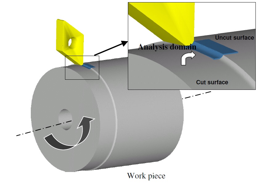
Basic components of Turning and it’s relation to analysis domain
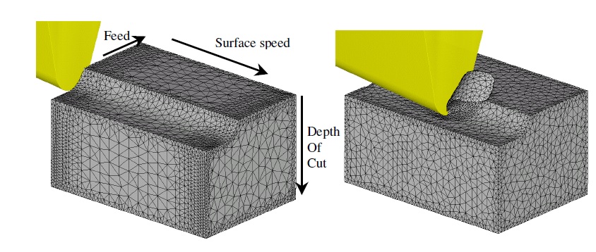
Simulation model and basic cutting parameters definition
Starting the 3D machining wizard
We can open 3D Cutting wizard in two ways:
a. Create a new problem either by selecting File![]() **New Problem** or by clicking the New Problem
**New Problem** or by clicking the New Problem ![]() icon. The Problem Setup window will appear. Select “ Integrated Manufacturing Process “ radio button and Unit system as “SI “ using radio button. Define Problem Name as “3D_cutting “ and and make sure the “Show option dialog ” check box is turned on (if we do not turn on the “Show option dialog ” check box, then we will not get the New Project dialog in MO UI). Then click on
icon. The Problem Setup window will appear. Select “ Integrated Manufacturing Process “ radio button and Unit system as “SI “ using radio button. Define Problem Name as “3D_cutting “ and and make sure the “Show option dialog ” check box is turned on (if we do not turn on the “Show option dialog ” check box, then we will not get the New Project dialog in MO UI). Then click on ![]() button to open a new Problem using the Deform Integrated Manufacturing Process.
button to open a new Problem using the Deform Integrated Manufacturing Process.
Multiple operation wizard will open with the New Project dialog, at this point user will be prompted to specify a project name (system will create a separate folder with this project name) and title for this session. In this session we will use “3D_cutting “ as the project name. Click on ![]() to continue to open the operation. MO wizard will open, add 3D Cutting operation from the Explorer Operations list. Add the operation by clicking on
to continue to open the operation. MO wizard will open, add 3D Cutting operation from the Explorer Operations list. Add the operation by clicking on ![]() button available next to 3D Cutting or by drag and drop into the Operation editor.
button available next to 3D Cutting or by drag and drop into the Operation editor.
b. Create a new problem either by selecting File![]() **New Problem** or by clicking the NewProblem
**New Problem** or by clicking the NewProblem![]() **icon. The Problem Setup window will appear. Select “ **3D Cutting “ radio button and Unit system as “SI “ using radio button (see Fig. 3DTL1.3.). Define Problem Name as “ 3D_cutting “ and click on
**icon. The Problem Setup window will appear. Select “ **3D Cutting “ radio button and Unit system as “SI “ using radio button (see Fig. 3DTL1.3.). Define Problem Name as “ 3D_cutting “ and click on ![]() button to open a new Problem with 3D Cutting operation in MO wizard.
button to open a new Problem with 3D Cutting operation in MO wizard.
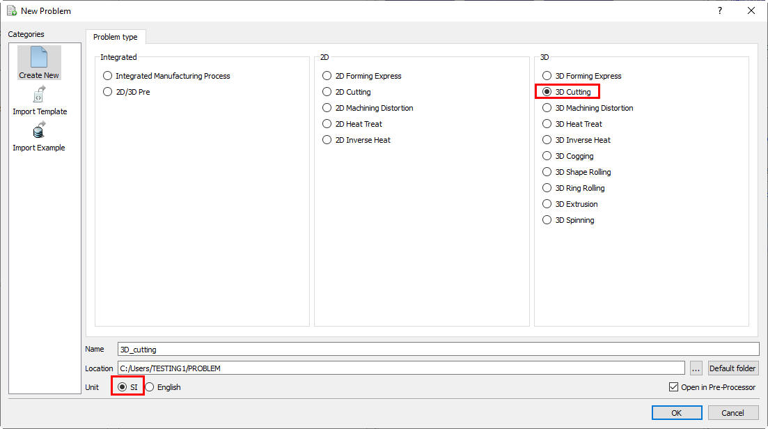
New Problem Setup Page
Define Machining Process data
In this lab we go through a typical setup with process conditions as follows
-
Material used: AISI 1045 Steel, Initial temperature = 20C.
-
Insert used: TNMA332 (uncoated, WC as base material), Tool holder: DTGNL
-
Process: Cutting speed = 250 mm/sec, Feed = 0.35 mm/rev, Depth of cut = 0.3 mm
Under the ‘Process ’ menu, Select Cutting type as ‘Turning ‘, enter the Environment temperature as 20 °C and use default Convection coefficient 0.02 N/sec/mm/C. Define ‘Cutting**speed(v) as **250mm/sec , feed rate (f) as 0.35mm/rev and Depth of cut (d) as 0.3 mm(see Fig. 3DTL1.4.). Alternatively user can also specify rotational speed of the workpiece and part diameter instead of surface speed. Then click ![]() until Tool page.
until Tool page.
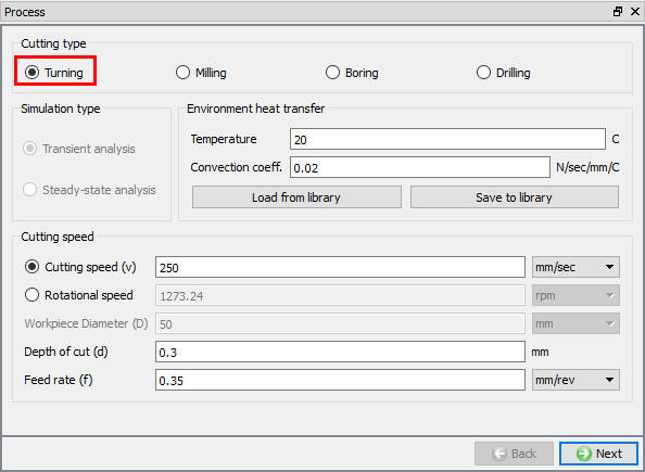
Process page
Defining Insert geometry
In ‘Tool ’ page, enter the tool temperature as 20°C. User can import the cutting edge geometry from a previously defined simulation keyword file or a database file using Import Object option. For this lab we will define the cutting edge geometry using the primitives available within the system. Click ![]() to enter the ‘Insert Geometry’ page and click on
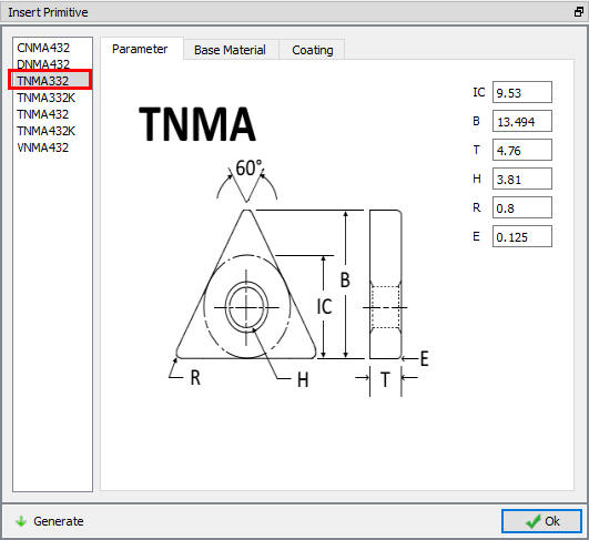
to enter the ‘Insert Geometry’ page and click on ![]() . Select TNMA332 geometry on the Insert Primitive page ( Fig. 3DTL1.5.), Once the insert is identified the user can check the basic parameters of this insert, the base material details and coatings, if any. Click on
. Select TNMA332 geometry on the Insert Primitive page ( Fig. 3DTL1.5.), Once the insert is identified the user can check the basic parameters of this insert, the base material details and coatings, if any. Click on ![]() to create insert geometry. Then click on
to create insert geometry. Then click on ![]() to come out of the ‘Geometry Primitive’ page and click on
to come out of the ‘Geometry Primitive’ page and click on ![]() to proceed.
to proceed.
Tool geometry primitives
Defining Tool Holder
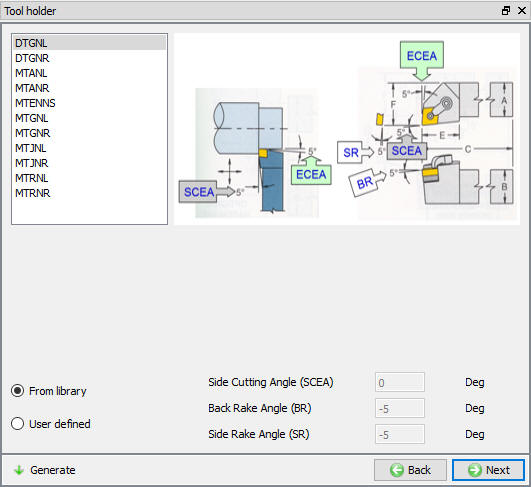
For the selected insert, the corresponding tool holders can be loaded from the tool holder library, or a new tool holder can be defined by providing basic cutting angles. For the insert TMNA332, the wizard will indicate the available holders from the library. Load the holder DTGNL from the library ( Fig. 3DTL1.6.). Basic cutting angles that are inherited from the tool holder data are SCEA (side cutting edge angle or the lead angle), BR (back rake angle) and SR (side rake angle). These basics angles and the process data (feed rate and depth of cut) control the correct position of the insert with respect to the work piece. Click the ![]() button to create the tool holder. Click
button to create the tool holder. Click ![]() .
.
Insert loading options
Assigning Insert material
In Material window, Selected insert base material will be loaded to material list from library while creating Tool geometry. So select ‘WC ‘ material from the list. click on ![]() to generate mesh for insert.
to generate mesh for insert.
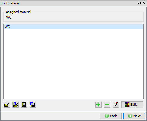
Assigning insert Material page
Generating insert mesh
In the ‘Tool Mesh Generation’ page select the ‘Use relative mesh size ‘ option, set the size ratio as 4 , and set the target number of tetrahedral elements to 45000. Generate the mesh by clicking ![]() . With the cutting edge information being part of the insert data, the wizard automatically applies a finer mesh near the cutting zone. Click
. With the cutting edge information being part of the insert data, the wizard automatically applies a finer mesh near the cutting zone. Click ![]() .
.
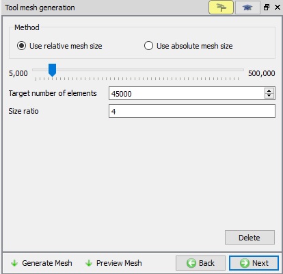
Insert Mesh page
Insert Boundary Conditions
By default Heat exchange with environment BCC will be assigned for whole surface, if not assign manually. Click ![]() .
.
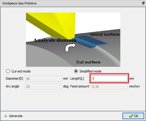
Workpiece Geometry
In the ‘Workpiece setup ’ define workpiece as a plastic object and temperature as 20 °C and click on ![]() to proceed.
to proceed.
Click on ![]() label in the ‘Workpiece Geometry’ page. In Primitive, specify the workpiece details. Depending upon the work piece diameter user can specify either a flat model or a curved model. The template will prompt for the related data, and will generate the work piece setup in the display area. For the current lab we use a ‘simplified model ’ with 7 mm length click on
label in the ‘Workpiece Geometry’ page. In Primitive, specify the workpiece details. Depending upon the work piece diameter user can specify either a flat model or a curved model. The template will prompt for the related data, and will generate the work piece setup in the display area. For the current lab we use a ‘simplified model ’ with 7 mm length click on ![]() to create the workpiece geometry (see Fig. 3DTL1.9.). Click
to create the workpiece geometry (see Fig. 3DTL1.9.). Click ![]() to close this geometry menu and click
to close this geometry menu and click ![]() to go to Material page.
to go to Material page.
Defining Workpiece geometry
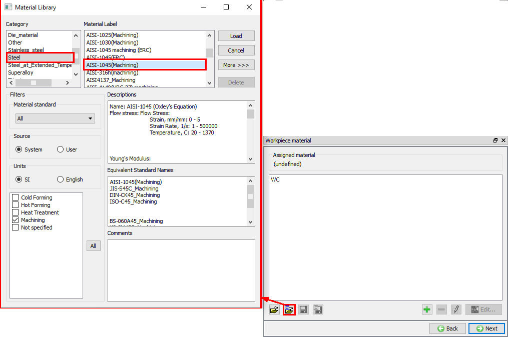
Assigning Workpiece Material
In ‘Workpiece material’ page, choose the option ‘import material from library’ ![]() option, select ‘Steel ’ category and ‘AISI-1045 (machining) ’ (see Fig. 3DTL1.10.). Click on
option, select ‘Steel ’ category and ‘AISI-1045 (machining) ’ (see Fig. 3DTL1.10.). Click on ![]() to this material and click
to this material and click ![]() to generate Mesh.
to generate Mesh.
Loading Workpiece material form Library
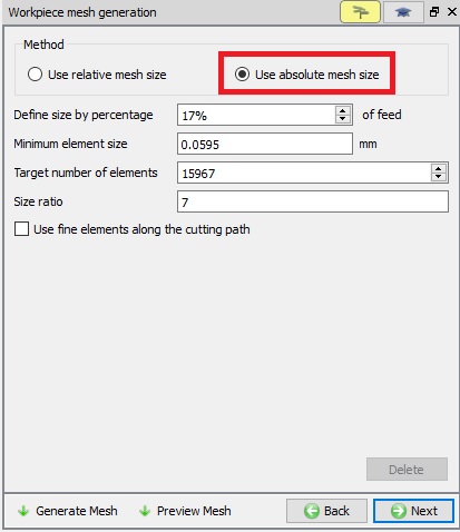
Generating mesh for Workpiece
After the work piece geometry is generated, generate mesh with element sizeratio of 7 , and minimum element size of 0.0595 mm. ( Fig. 3DTL1.11.) Click on ![]() to complete mesh generation for the workpiece. Click on
to complete mesh generation for the workpiece. Click on ![]() to BCC page.
to BCC page.
Workpiece Mesh page
Workpiece Boundary Condition page
In the ‘Workpiece BCC’ menu, check the boundary conditions imposed on workpiece by the system (see Fig. 3DTL1.12.), and click ![]() to Controls page. Note the velocity BCC assigned to the bottom surfaces away from the cutting surfaces to prevent workpiece from flying. Heat Exchange with BCC is assigned to all surfaces and temperature BCC is assigned for all surfaces except cutting surfaces.
to Controls page. Note the velocity BCC assigned to the bottom surfaces away from the cutting surfaces to prevent workpiece from flying. Heat Exchange with BCC is assigned to all surfaces and temperature BCC is assigned for all surfaces except cutting surfaces.
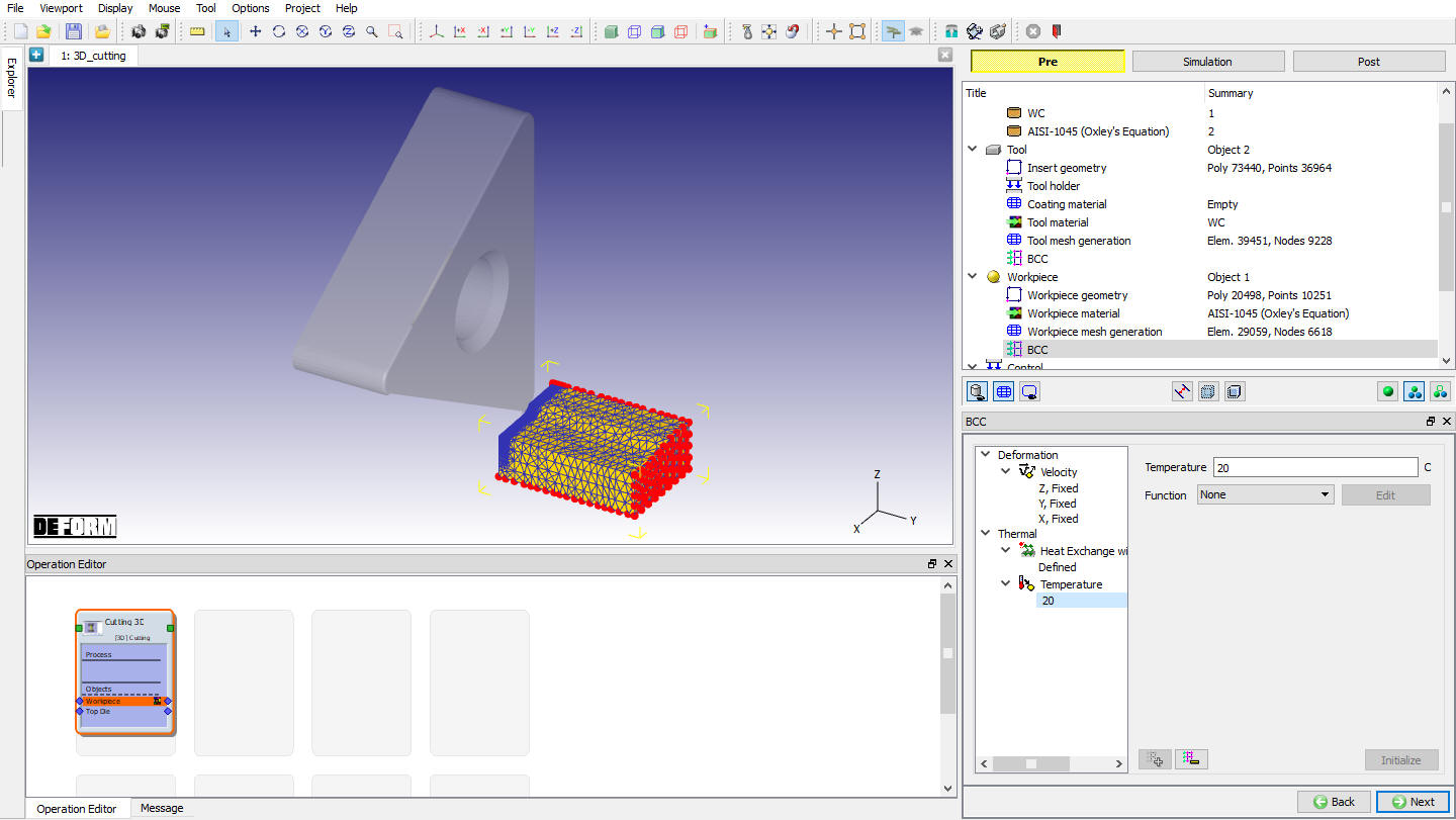
Assigned Temperature Boundary Condition for workpiece
Tool Positioning
In the Controls menu, click on ![]() . Check the position of Insert. If Insert is not in contact with workpiece, using interference method position the Insert and click
. Check the position of Insert. If Insert is not in contact with workpiece, using interference method position the Insert and click ![]() .
.
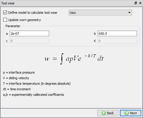
Tool Wear Setting
Select Usui’s model, the coefficients used in this model should be determined based on experimental calibration as they depend on the process conditions and the materials used for accurate results. As an example for this case we use a = 0.0000002 and b = 650.5 (see Fig. 3DTL1.13.). Click ![]() to contact page.
to contact page.
Tool wear setup window
Contact page
In Contact page, use default relations. Click on Tool - Workpiece relation Edit button and define shear friction factor as0.5 and the interfaceheattransfer coefficient as 45 N/sec/mm/C (as shown in Fig. 3DTL1.14.), click on ![]() to generate contacts. Click on
to generate contacts. Click on ![]() to Step Control page.
to Step Control page.
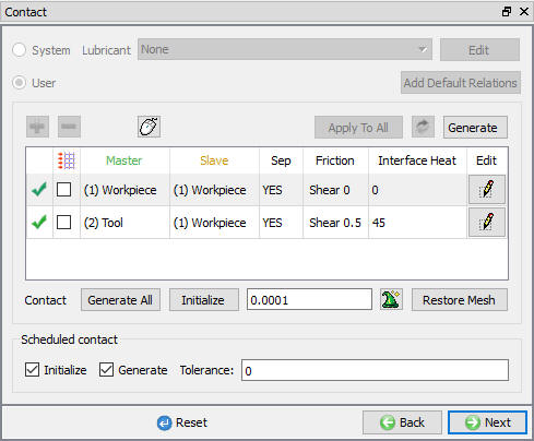
Contact page
Step Control page
Check the ‘Simulation Controls’ and set the length of cut as ‘3.5 mm ’ and leave the rest as default values and proceed to generate the Database.
Generate Database
In Generate DB page. Click on the ![]() button to generate the database. Observe the message in Message tab informing database generation status.
button to generate the database. Observe the message in Message tab informing database generation status.
Running Simulation
Once the database has been generated switch to the Simulation mode by clicking on ![]() button above the operation tree. Click on the
button above the operation tree. Click on the ![]() action label to open the Run Options dialog as shown in Fig. 3DTL1.15. Use the default ContinueRun option to select “Continue from the last step ” option and then select the Simulation mode as Interactive radio button. Click on
action label to open the Run Options dialog as shown in Fig. 3DTL1.15. Use the default ContinueRun option to select “Continue from the last step ” option and then select the Simulation mode as Interactive radio button. Click on ![]() button to run the simulation.
button to run the simulation.
To define MPI settings, click on ![]() button, Run Options window will expand and displays options to define MPI settings for simulation (max number of processors that can be defined depend on your 3D MPI license).
button, Run Options window will expand and displays options to define MPI settings for simulation (max number of processors that can be defined depend on your 3D MPI license).
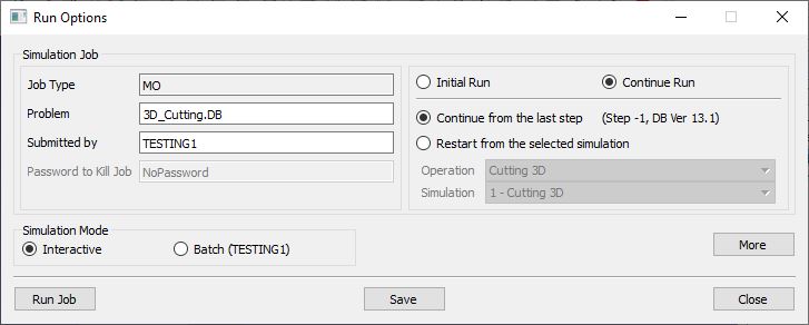
Run Simulation Window
Monitor the progress of the simulation by looking at the Simulation Message and Simulation Log tab, making sure that the ![]() option is checked. User can view the cutting process as the simulation proceeds to the specified cutting length from Simulation graphics.
option is checked. User can view the cutting process as the simulation proceeds to the specified cutting length from Simulation graphics.
Post Processing
When the simulation is completed, review the results by switching to Post mode using the ![]() button above the Simulation tool bar.
button above the Simulation tool bar.
Play through the steps of the simulation and look how the chip has been formed during cutting process.
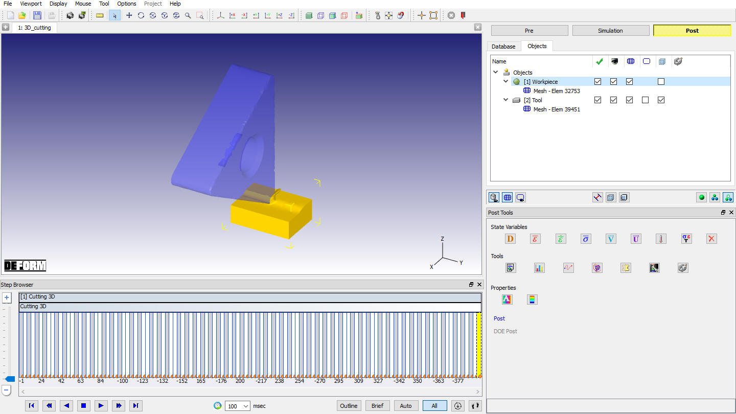
MO Post mode
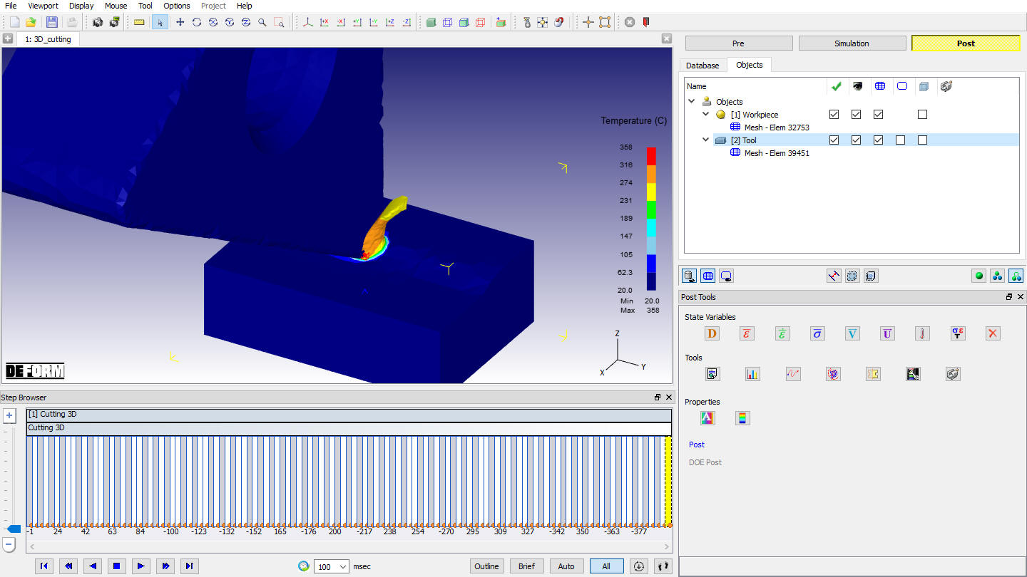
Temperature distribution in workpiece and Tool
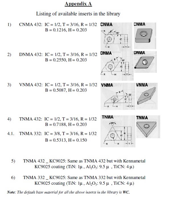
Appendix A
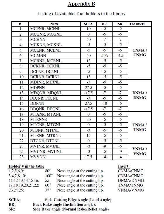
Appendix B
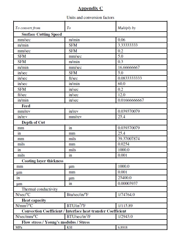
Appendix C