Cogging Lab1
1.1. Introduction
1.2. Problem Setup
1.3. Define Process settings
1.4. Define Pass Table
1.5. Load material
1.6. Define Object
1.7. Define Billet Object
1.8. Define Top Die
1.9. Define Manipulator data
1.10. Object Positioning
1.11. Scheduled Positioning
1.12. Define Inter-object relation
1.13. Simulation Preview
1.14. Simulation Controls
1.15. Database Generation
1.16. Running Simulation
1.17. Post Processing
Introduction
Cogging wizard provides options such as pass table, movement controls, reheating options and primitives for dies, billets and manipulators, with these options user can set up typical cogging process with ease. Cogging can be accessed from DEFORM MO wizard, which can be accessed from the DEFORM GUI Main.
Problem Setup
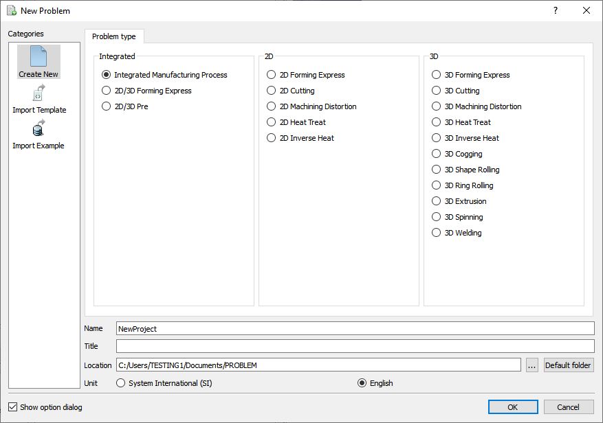
Create a new problem either by selecting File ![]() New Problem or by clicking the New Problem
New Problem or by clicking the New Problem ![]() icon. The Problem Setup window will appear as shown in Fig. 3DCGL1.1. Select “Integrated Manufacturing Process “ radio button and unit system as “English “ radio button in unit field. Define Problem Name as “Coglab “ and make sure the “Show option dialog” check box is turned on (if we do not turn on the “Show option dialog ” check box, then we will not get the New Project dialog in MO UI). Then click on
icon. The Problem Setup window will appear as shown in Fig. 3DCGL1.1. Select “Integrated Manufacturing Process “ radio button and unit system as “English “ radio button in unit field. Define Problem Name as “Coglab “ and make sure the “Show option dialog” check box is turned on (if we do not turn on the “Show option dialog ” check box, then we will not get the New Project dialog in MO UI). Then click on ![]() button to open a new Problem using the Deform Integrated Manufacturing Process.
button to open a new Problem using the Deform Integrated Manufacturing Process.
Problem type selection window
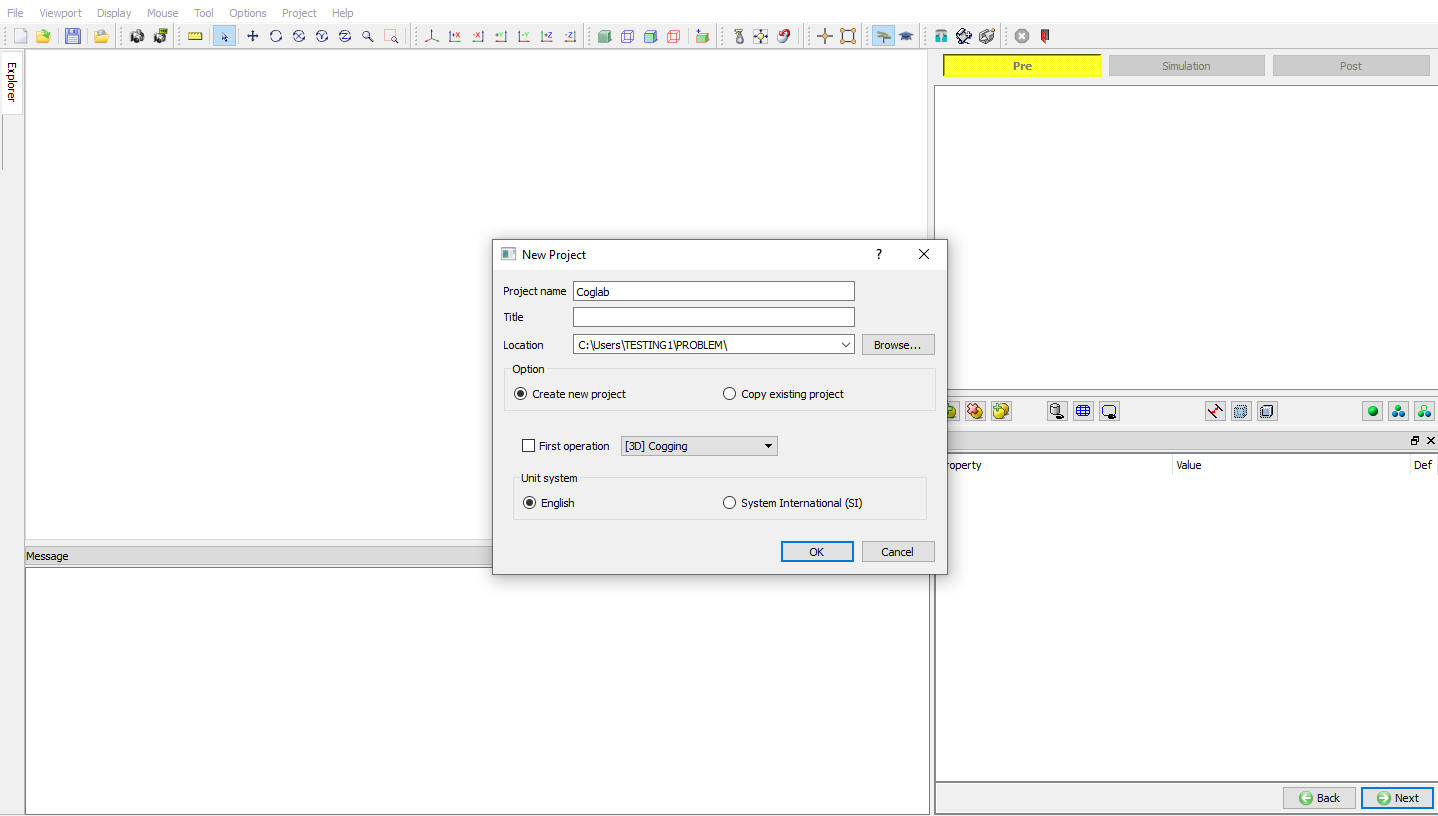
Multiple operation wizard will open with the New Project dialog, In this session we use ‘Coglab ’ as the project name. 3D Cogging operation can also be added in “New Project” dialog, in this lab we will add Cogging operation from Explorer operation list, so do not check “First operation” check box and “Cogging” operation in “New Project” dialog. Click on ![]() to continue to open the operation. MO wizard will open (see Fig. 3DCGL1.2.).
to continue to open the operation. MO wizard will open (see Fig. 3DCGL1.2.).
Assigning problem name
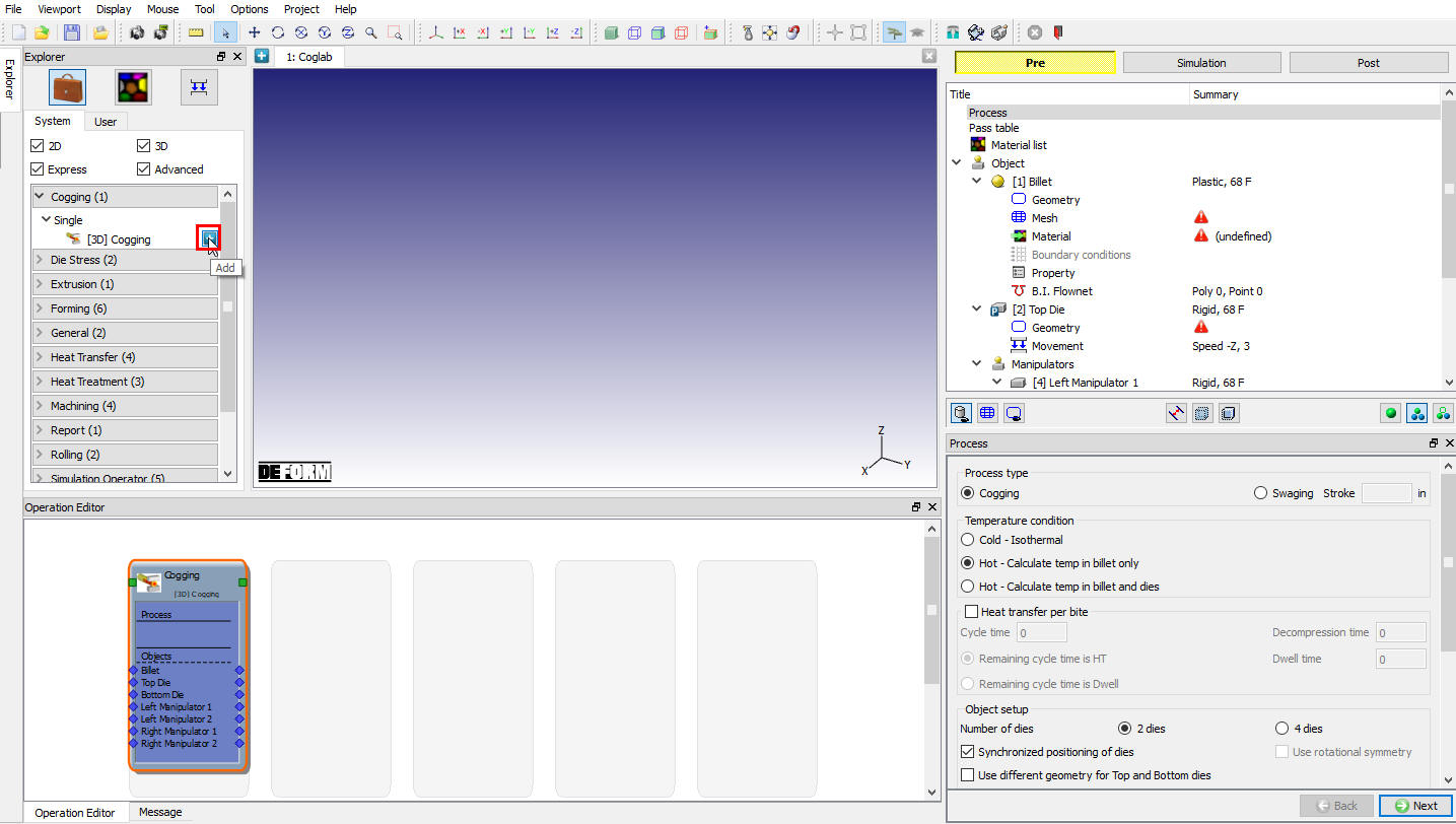
Add 3D Cogging operation from the Explorer Operations list. Add the operation by clicking on ![]() button available next to 3D Cogging or user can also add by drag and drop into the Operation Editor (see Fig. 3DCGL1.3.). When we add the Cogging operation, process Window will open by default.
button available next to 3D Cogging or user can also add by drag and drop into the Operation Editor (see Fig. 3DCGL1.3.). When we add the Cogging operation, process Window will open by default.
Operation Explorer
Define Process settings
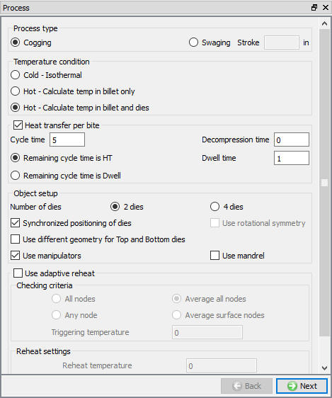
In Process window, select the Hot - Calculate temp in Billetanddies radio button and turn on Heat transfer per bite check box, as we will be setting up non isothermal process. Define Cycle time as 5 sec and Dwell time as 1 sec as shown in Fig. 3DCGL1.4.
In process page, user can select the 2 dies or 4 dies for the simulation and also user can decide whether to use manipulators or not for holding the billet (or apply direct BCC to the billet). User can use Mandrel for hollow billets as in case of swaging process. This window also has options to set reheating criteria using Adaptive Reheating. For this lab we will use 2 dies and Manipulators, click on ![]() to pass table.
to pass table.
Process window
Define Pass Table
In pass table window, we will define the Axial feed per bite, Cross section thickness, movement Direction, Rotation per bite (Deg), Rotation per Pass (Deg).
For this particular lab, we will be defining two passes and we will use Auto Bite calculation. So just add one more pass using ![]() then click on Pass 1. (See Fig. 3DCGL1.5.)
then click on Pass 1. (See Fig. 3DCGL1.5.)
Tip :
In order to save time for setting data for each pass, what you can do is just define the first pass and then add the next pass. It will copy all the data from the first pass to the next one.
Turn on the Auto calculate Bites check box so that system calculates the number of bites required for the pass automatically based on the billet length or conditions mentioned in die start and stop position.
Axial feed per bite as 10 inch,
Cross section thickness as 18 inch and
Movement direction as –X for dies.
For second pass you can change the rotation per pass (Deg) to 90 with all the other parameters same as that of pass 1. Keep all the other values to default values and click on ![]() to Material page.
to Material page.
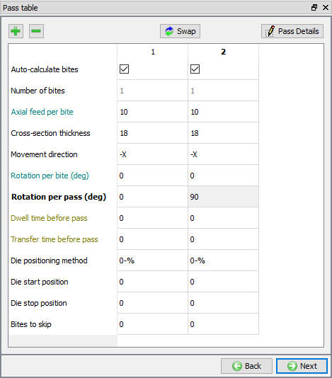
Pass table window
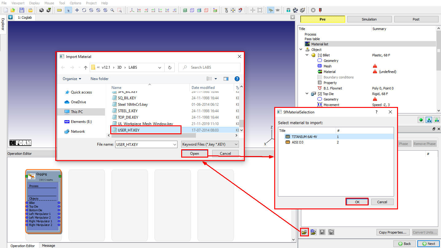
Load material
For this lab we will be using material from USER_HT.KEY file available in installation path Labs Directory. In material list window, select the import Material data from a file ![]() option and a dialog will open, browse to USER_HT.KEY file from Labs Directory and open. A material selection dialog will be opened, select the TITANIUM 6Al-4V click
option and a dialog will open, browse to USER_HT.KEY file from Labs Directory and open. A material selection dialog will be opened, select the TITANIUM 6Al-4V click ![]() to import the material. Repeat the same procedure to import the Die material AISI D3 available in USER_HT.KEY file. (see Fig. 3DCGL1.6.). Click on
to import the material. Repeat the same procedure to import the Die material AISI D3 available in USER_HT.KEY file. (see Fig. 3DCGL1.6.). Click on ![]() .
.
Material window
When we click ![]() , the properties of the materials loaded into the material list page will be displayed which can be edited (see Fig. 3DCGL1.7.). In this lab as we going to retain the default values, click
, the properties of the materials loaded into the material list page will be displayed which can be edited (see Fig. 3DCGL1.7.). In this lab as we going to retain the default values, click ![]() until object page.
until object page.
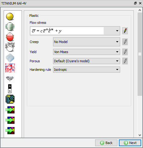
Material Properties page
Define Object
In object window, options are provided to maintain the mesh size on billet during simulation either by aspect ratio or element size. For detail description of these options, refer Cogging Manual. User is also provided with a choice to perform billet straightening between passes or between bites. Billet straightening is a geometry manipulation operation performed in order to avoid the excessive bending caused by slight positioning error accumulated over multiple passes. For this lab we will not be doing any billet straightening (see Fig. 3DCGL1.8.). Click ![]() .
.
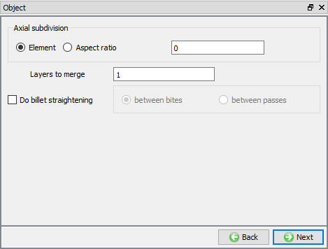
Object window
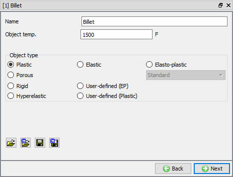
Define Billet Object
In Billet window, change the objecttemperature to 1500 °F from 68°F (see Fig. 3DCGL1.9.). Click ![]() .
.
Billet window
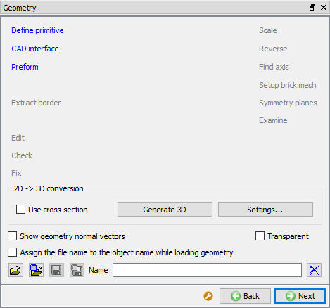
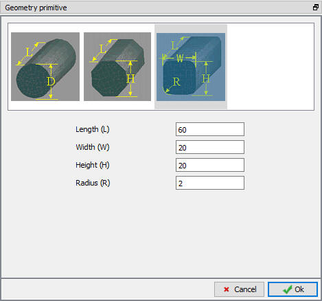
Define Billet Geometry
In billet geometry window, select the ![]() option as we will be constructing billet geometry from primitives. In Primitive window choose the round cornered rectangle as the cross section and enter a height/width of 20 , a length of 60 and a cornerradius of 2 (see Fig. 3DCGL1.11.). After creating geometry from primitive, make sure in Geometry page “Use cross section” check box in 2D => 3D Conversion options is checked. Cogging operation uses 2D cross section to generate brick mesh and cross section is updated through out the simulation hence “ Use cross section” check box in 2D=> 3D Conversion options should always be kept checked in Cogging operation. Click
option as we will be constructing billet geometry from primitives. In Primitive window choose the round cornered rectangle as the cross section and enter a height/width of 20 , a length of 60 and a cornerradius of 2 (see Fig. 3DCGL1.11.). After creating geometry from primitive, make sure in Geometry page “Use cross section” check box in 2D => 3D Conversion options is checked. Cogging operation uses 2D cross section to generate brick mesh and cross section is updated through out the simulation hence “ Use cross section” check box in 2D=> 3D Conversion options should always be kept checked in Cogging operation. Click ![]() .
.
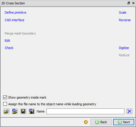
2D cross section of the geometry will be displayed as shown in figure. The 2D cross section can be edited if required using options available in 2D cross section page (see Fig. 3DCGL1.12.). In this lab the 2D cross section will not be edited, hence click ![]() .
.
Geometry window
Billet primitive window
2D geometry window
Define Billet mesh
In mesh page, enter 100 as the number of mesh elements for 2D cross-section and sizeratio as 1. Enter 14 as the numberoflayers along the axial direction. Click on the ![]() button and click on
button and click on ![]() in “Default Boundary condition” popup. Enter 25000 for re-meshing number of elements. This number will be used to generate tetrahedral mesh in case brick re-meshing fails because of too much distortion (see Fig. 3DCGL1.13.). Click
in “Default Boundary condition” popup. Enter 25000 for re-meshing number of elements. This number will be used to generate tetrahedral mesh in case brick re-meshing fails because of too much distortion (see Fig. 3DCGL1.13.). Click ![]() .
.
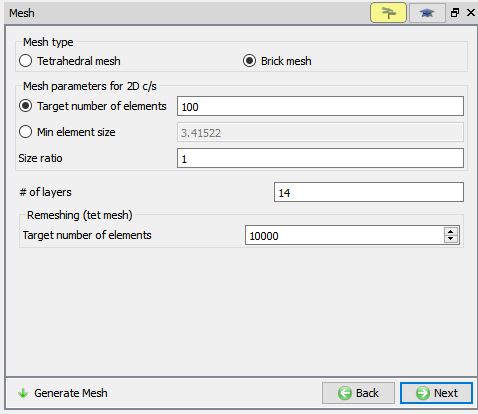
Billet mesh window
Assign Billet Material
In Billet material page, select TITANIUM 6Al-4V material for billet that was imported earlier (see Fig. 3DCGL1.14.). Click ![]() .
.
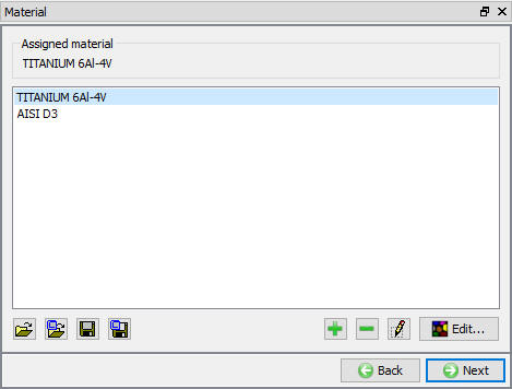
Material window
Define Boundary condition
Depending on the process conditions selected, system will generate BCC automatically for thermal and symmetry. In this lab we are not using symmetry, hence only thermal BCC are generated automatically as shown in Fig. 3DCGL1.15. For this lab we will keep the default generated BCC. Click ![]() .
.
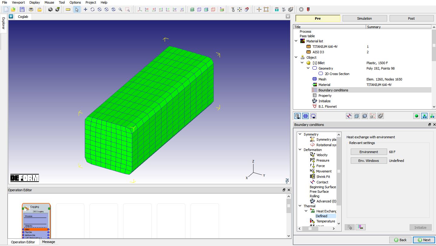
Billet BCC window
Billet Properties
Miscellaneous object parameters which affect either thermo-mechanical behavior of the object, or numerical solution behavior, are specified in the Object-Properties window (see Fig. 3DCGL1.16.). For this lab we do not require to make any changes in property window. Click ![]() until Top die page.
until Top die page.
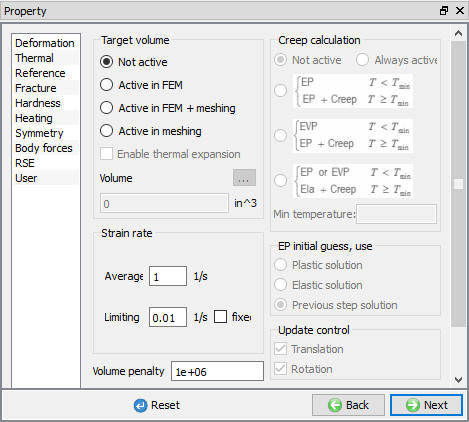
Billet property window
Define Top Die
In Top die Window, change the object temperature to 200° F from 68° F (see Fig. 3DCGL1.17.). Click ![]() .
.
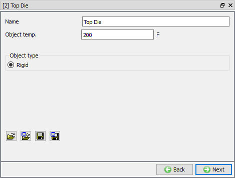
Top die window
Define Top Die Geometry
We will be using primitive geometry options provided in wizard to define die geometry hence, select the ![]() option and in Primitive window enter a height/width of 15 , a length of 25 and a cornerradius of 2(see Fig. 3DCGL1.18.). Click
option and in Primitive window enter a height/width of 15 , a length of 25 and a cornerradius of 2(see Fig. 3DCGL1.18.). Click ![]() .
.
In this lab the 2D cross section will not be edited, hence click ![]() .
.
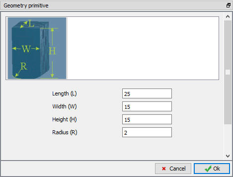
Top die Geometry Window
Define Top Die Mesh
In mesh page, enter 100 as number of 2D cross-section mesh elements and sizeratio as1. We will have 7 layers in axial direction (see Fig. 3DCGL1.19.). Click on the ![]() button to generate mesh for die and click on
button to generate mesh for die and click on ![]() in “Default Boundary condition” popup. The die geometry and mesh is duplicated for other die also. Click
in “Default Boundary condition” popup. The die geometry and mesh is duplicated for other die also. Click ![]() .
.
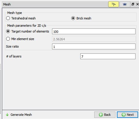
Top die Mesh window
Define Top Die Material
In Top die material page, select AISI D3 for top die (see Fig. 3DCGL1.20.). Click ![]() .
.
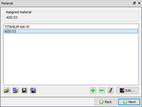
Top die material window
Define Top Die movement
In Top die movement page, Change Die Speed to 1 inch/sec for this lab (see Fig. 3DCGL1.21.). User also have an option to use mechanical press and other type of movement controls like screw press from Advanced option based on the process requirement. Click ![]() until manipulator page.
until manipulator page.
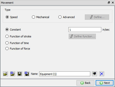
Top die movement window
Define Manipulator data
In manipulator window, change the lefthandoverdistance to 10 inch and righthandoverdistance to 10 inch. The handover distance helps in release of one set of manipulators while other set comes into action. For these settings the Manipulators set are released when dies are within 10in from manipulator set. The dampening conditions for spring loaded manipulators can be set as shown in Fig. 3DCGL1.22. From DEFORM V12, “Generate manipulator BCC “ option has been added in Manipulators page, when user turns on this check box then contact BCC will be generated with manipulator for all surface nodes (manipulator contact region) within friction window. Click ![]() .
.
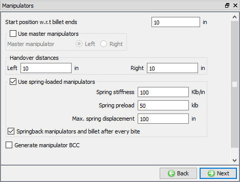
Manipulator window
Define Left manipulator object
In Left manipulator Window, change the object temperature to 200° F from 68°**F (see Fig. 3DCGL1.23.). Click ![]() .
.
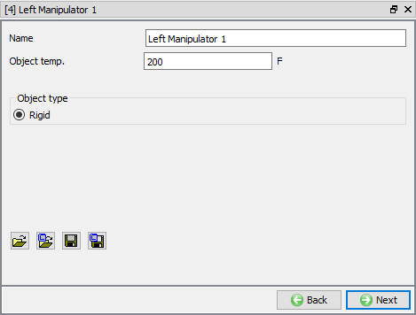
Left manipulator window
Define Left manipulator Geometry
In Left manipulator geometry page select the ![]() option to define manipulator geometry from primitives, in Primitive window enter dimensions as shown in Fig. 3DCGL1.24. and create the geometry and click
option to define manipulator geometry from primitives, in Primitive window enter dimensions as shown in Fig. 3DCGL1.24. and create the geometry and click ![]() .
.
In this lab the 2D cross section will not be edited, hence click ![]() until mesh page.
until mesh page.
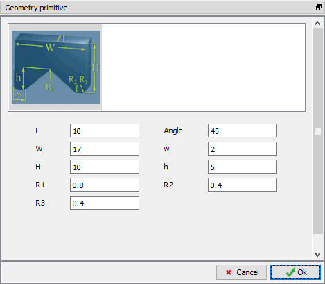
Manipulator primitive window
Define Left manipulator Mesh
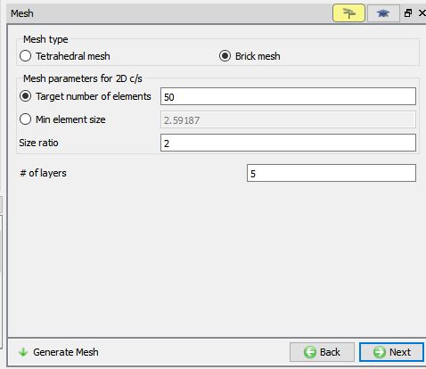
In mesh page, enter 50 as number of 2D cross-section mesh elements and sizeratio as 2. We will have 5 layers in axial direction. Click on the ![]() button to generate mesh for Manipulator and click on
button to generate mesh for Manipulator and click on ![]() in “Default Boundary condition” popup. The manipulator geometry and mesh is duplicated for other manipulators also (see Fig. 3DCGL1.25.). Click
in “Default Boundary condition” popup. The manipulator geometry and mesh is duplicated for other manipulators also (see Fig. 3DCGL1.25.). Click ![]() .
.
Left manipulator mesh window
Define Left manipulator Material
In Left manipulator material page, select AISI D3 as material for Left manipulator (see Fig. 3DCGL1.26.). Click ![]() to positioning page.
to positioning page.
Assigning Material window
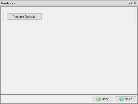
Object Positioning
Positioning of the objects is controlled by the system automatically depending on the pass details set in pass table. Hence we do not require any positioning to be done click ![]() to Scheduled positioning page.
to Scheduled positioning page.
Positioning window
Scheduled Positioning
Since no positioning to be done, click ![]() even in Scheduled positioning page.
even in Scheduled positioning page.
Define Inter-object relation
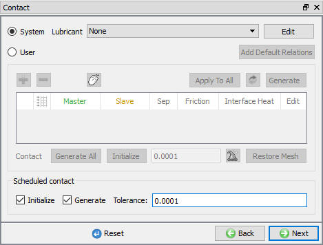
System will generate contact relations between the objects automatically, if user would like to define any other condition apart from default conditions then user option should be selected. For this lab we will use system generated contact conditions, select System contact definition type and check scheduled contact Initialize and Generate check boxes and enter small contact tolerance value 0.0001 as shown in (see Fig. 3DCGL1.28.). The inter-object Heat transfer coefficients and friction coefficient can be set in simulation controls page. Click ![]() .
.
Inter-object window
Simulation Preview
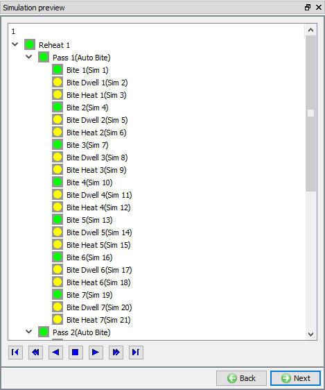
Simulation Preview provides an overview of the operations like deformation, dwelling, reheat..etc. to be executed based on the process definition as animation. It also gives preview of the setup at each operation. In Simulation preview window, by clicking the play buttons animation would be played (see Fig. 3DCGL1.29.). Click ![]() .
.
Simulation preview window
Simulation Controls
In simulation control window, define the number of steps as 10 for deformation simulation,step increment to save as 500 so that only one step is saved per bite, step definition stroke value as 0.1 in/step.
Heat transfernumber of steps and step increment as 10 so that only 1 step is stored for heat transfer operation like dwell. As several number of operations are executed before simulation of cogging is completed, the DB size is controlled by saving limited number of steps into DB. Keep all the other values to default and click ![]() . From v11.0 onwards, explicit solver is made available for cogging simulations however we will be using implicit solver for this lab (see Fig. 3DCGL1.30.).
. From v11.0 onwards, explicit solver is made available for cogging simulations however we will be using implicit solver for this lab (see Fig. 3DCGL1.30.).
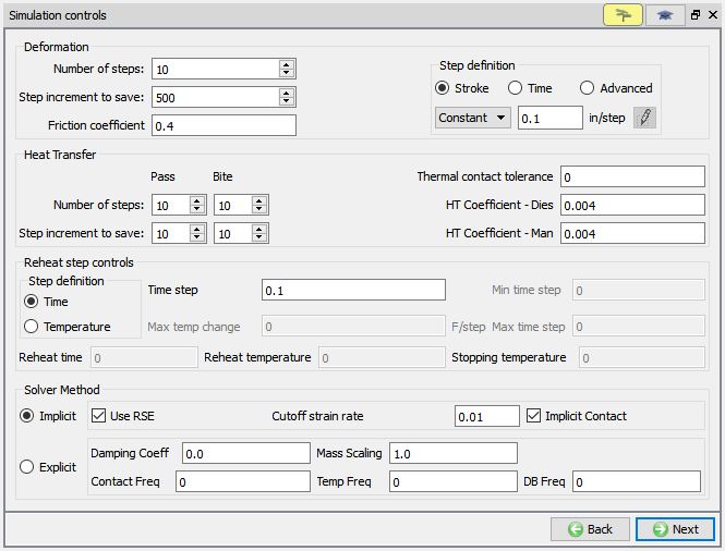
Simulation control window
Database Generation
In DB generation page, Click on ![]() action label to check the problem. Generate a database by clicking
action label to check the problem. Generate a database by clicking ![]() action label.
action label.
Once we click on ![]() action label, ProblemID.MST file is generated along with Database.
action label, ProblemID.MST file is generated along with Database.
Running Simulation
Once the database has been generated, switch to the Simulation mode by clicking on ![]() button above the operation tree. Click on the
button above the operation tree. Click on the ![]() action label to open the Run Options dialog as shown in Fig. 3DCGL1.31. Use the default Continue Run option to select “Continue from the last step ” (from step -1) option and then select the Simulation mode as Interactive and click on
action label to open the Run Options dialog as shown in Fig. 3DCGL1.31. Use the default Continue Run option to select “Continue from the last step ” (from step -1) option and then select the Simulation mode as Interactive and click on ![]() button to run the simulation.
button to run the simulation.
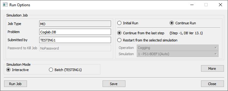
Run Simulation popup window
Monitor the progress of the simulation by looking at the Simulation graphics window, Simulation Message and Simulation Log tabs (see Fig. 3DCGL1.32.). Message file and log files are refreshed automatically for monitoring the simulation progress. Simulation graphics tool bar options can be used to plot basic state variables such as temperature, strain and contact for objects while simulating the problem. Also now Summary, Load-Stroke, Mirroring, Slicing and Measure options added in toll list we can use.
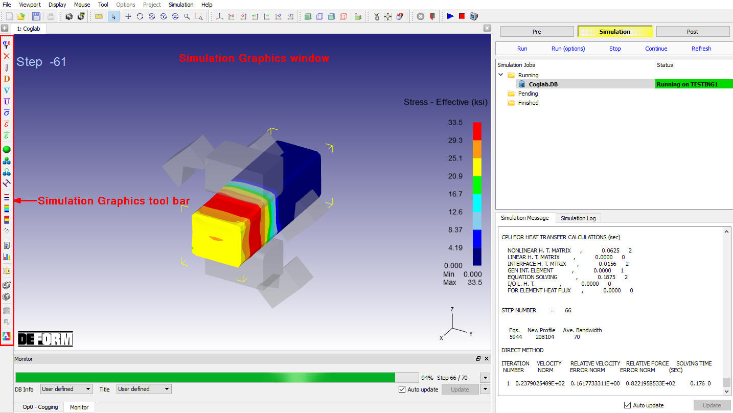
MO simulation mode
For cogging simulation, all simulation information of cogging while running will be written to ProblemID.MST file, ProblemID.MST file helps to run the cogging simulation sequentially each bite deformation and heat transfer operations as individual operations based on the settings in process page and pass table. ProblemID.MST controls the start and stop of each operation. For all operations, start and stop messages are showed in Message file. After the completion of the all operations, in Simulation Log file we will see message as “MULTIPLE OPERATION COMPLETED”.
Post Processing
When the simulation is complete, user can review the results by switching to Post mode using the ![]() button. (See Fig. 3DCGL1.33.)
button. (See Fig. 3DCGL1.33.)
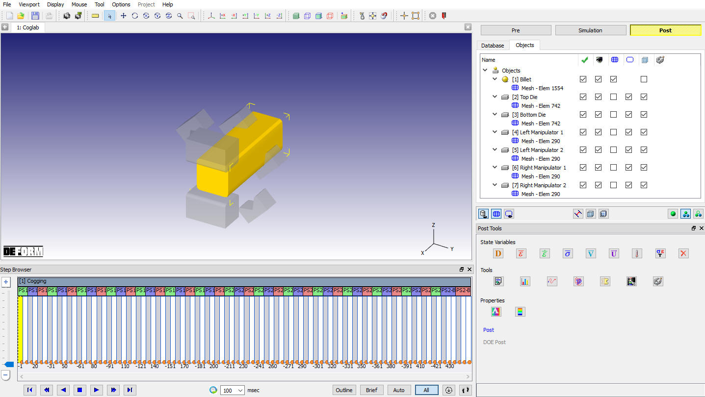
MO Post Mode
Play through the Steps and see the Temperature distribution and Strain distribution by plotting the Temperature and effective strain State variables.(see Fig. 3DCGL1.34.)
The temperature change in dies can also be noticed as shown in Fig. 3DCGL1.35.
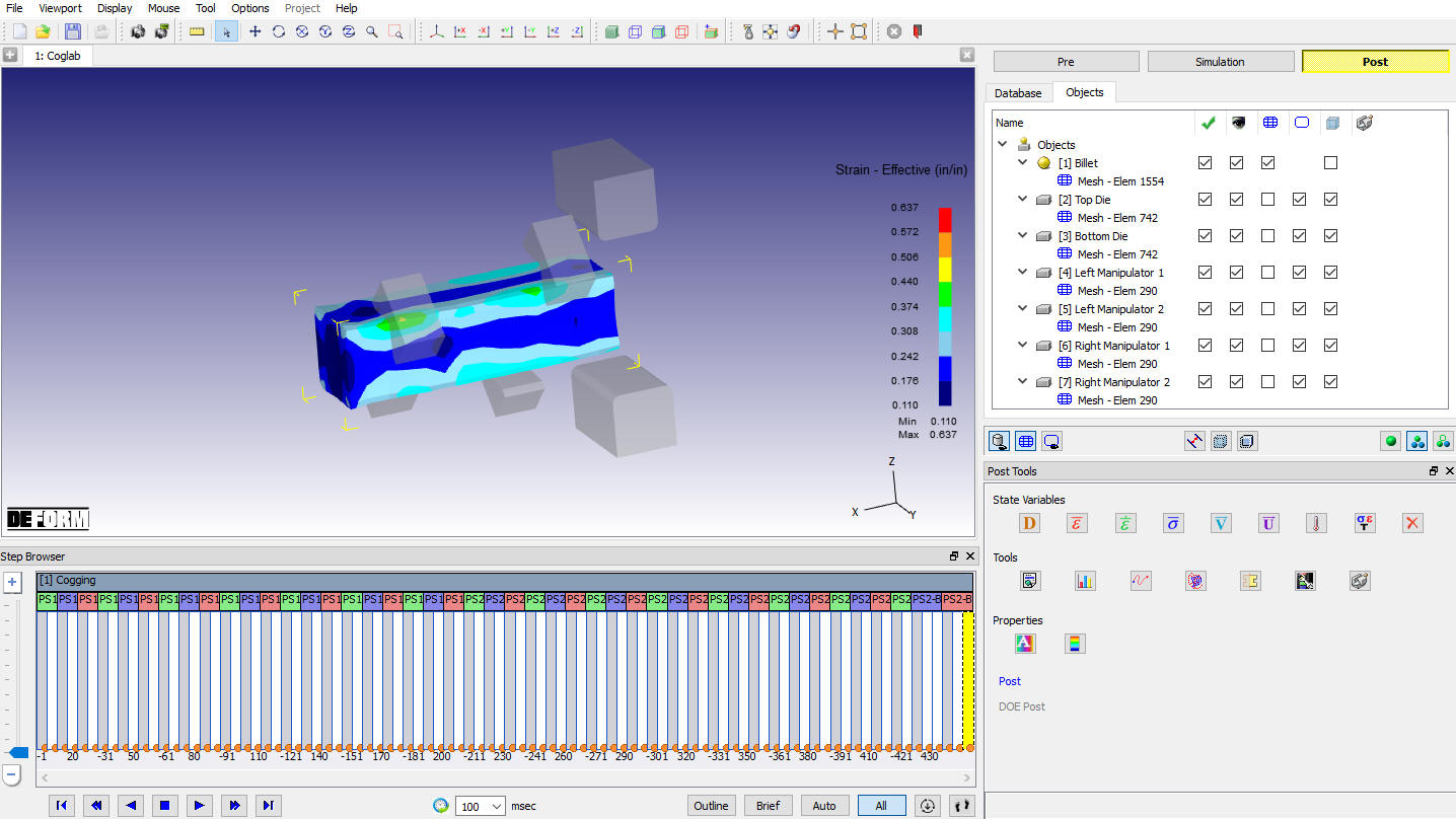
Strain Distribution
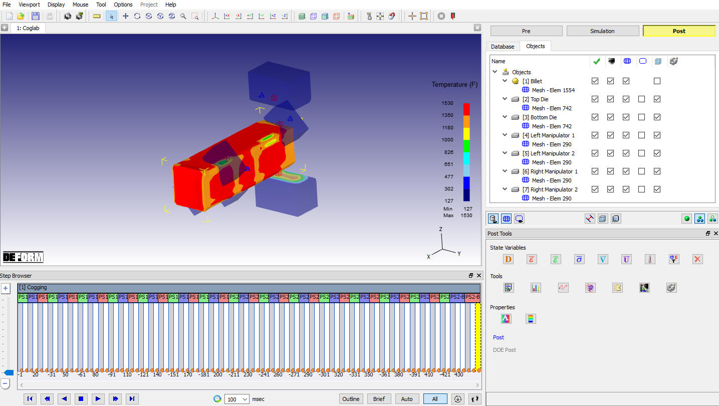
Temperature Distribution