2D Steady State Machining Lab

1.1. Problem Summary

1.2. Creating New Problem

1.3. Define Machining Process data

1.4. Loading Cutting tool Coating material

1.5. Defining Cutting Tool geometry

1.6. Coating definition

1.7. Assign Tool material

1.8. Generating Tool mesh

1.9. Tool Boundary conditions

1.10. Set the Workpiece geometry data

1.11. Assigning Workpiece material

1.12 Generating Mesh for workpiece

1.13. Workpiece Boundary condition page

1.14. Initialize

1.15. Tool wear Setting

1.16. Contact

1.17. Step Control

1.18. Generate Database

1.19. Running Simulation

1.20. Post Processing

Problem Summary

This lab will briefly demonstrate how to use the machining template to prepare model data representing orthogonal cutting conditions (cutting edge is orthogonal/perpendicular to the cutting direction) to simulate chip formation process. Interactive definition of the process conditions, cutting edge, coating, material, steady state and tool stress related features are discussed here. Brief description of the orthogonal cutting conditions and how the process parameters are related to the modeling domain are indicated as shown in the Fig. 2DSSL1.1.

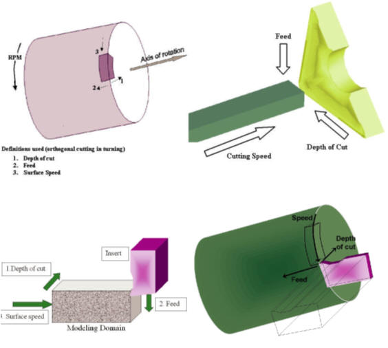
Relationship between the process data and analysis domain

Creating New Problem

We can open 2D Cutting wizard in two ways:

a. Create a new problem either by selecting File NewProblem or by clicking the NewProblem icon. The Problem Setup window will appear. Select “ Integrated Manufacturing Process “ radio button and Unit system as “SI “ using radio button. Define Problem Name as “2D_CUTTING_STEADY “ and click on button to open a new Problem using the Integrated Manufacturing Process. Multiple Operation wizard will open, at this point user will be prompted to specify a project name (system will create a separate folder with this project name) and title for this session. In this session we will use “2D_CUTTING_STEADY “ as the project name. Click on to continue to open the operation. Integrated Manufacturing Process will open, add 2D Cutting operation from the Explorer Operations list. Add the operation by clicking on button available next to 2D Cutting or by drag and drop into the Operation editor.**

b. Create a new problem either by selecting File **New**Problem or by clicking the New Problem icon. The Problem Setup window will appear. Select “2D Cutting” radio button and Unit system as “SI “ using radio button as shown in Fig. 2DSSL1.2. Define Problem Name as “ 2D_CUTTING_STEADY “ and click on button to open a new Problem with 2D Cutting operation in MO wizard.

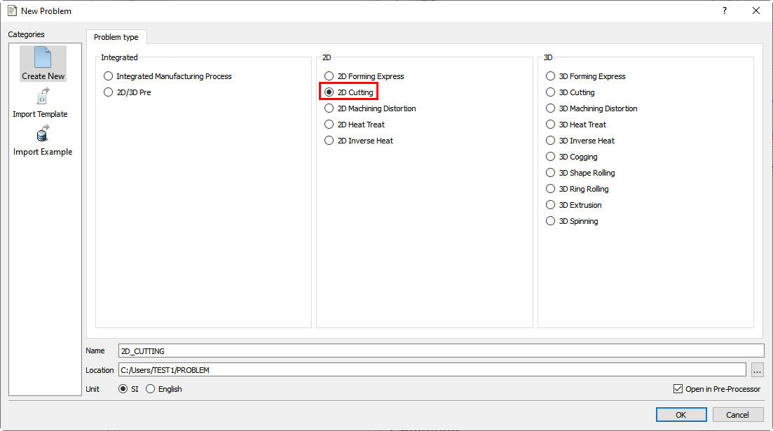
Problem Setup page

Define Machining Process data

Under the ‘Process ’ menu, Select Simulation type as ‘Steady-stateAnalysis ‘, enter the EnvironmentHeatTransfertemperature as 22.5 °C and use default Convection coefficient 0.02N/sec/mm/C. Select the ‘Surfacespeed as 250m/min and feedrate as 0.15mm/rev ’ (see Fig. 2DSSL1.3.). Alternatively user can also specify rotational speed of the workpiece and part diameter instead of surface speed. Then click on .

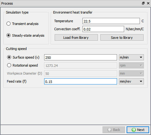
Process page

Loading Cutting tool Coating material

In Material List page, load ‘Coating-TiN’ and ‘Coating-Al2O3 ‘ Material from Tool_Material category for assigning to Tool coating. Then click on until Tool page.

Defining Cutting Tool geometry

In ‘Tool’ page, enter the tool temperature as 20°C. We can import the cutting edge geometry from a previously defined simulation keyword file or a database file using Import Object option. For this lab we will define the cutting edge geometry using the primitives available with the system. Click on to enter the ‘Insert Geometry’ menu (see Fig. 2DSSL1.4.) and click on . Select #3 geometry in Primitive page and use default geometry parameters. Click on to create geometry. Then click on to come out of ‘Geometry Primitive’ menu and click on to proceed.

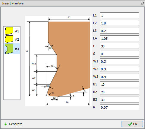
Insert Primitive Window

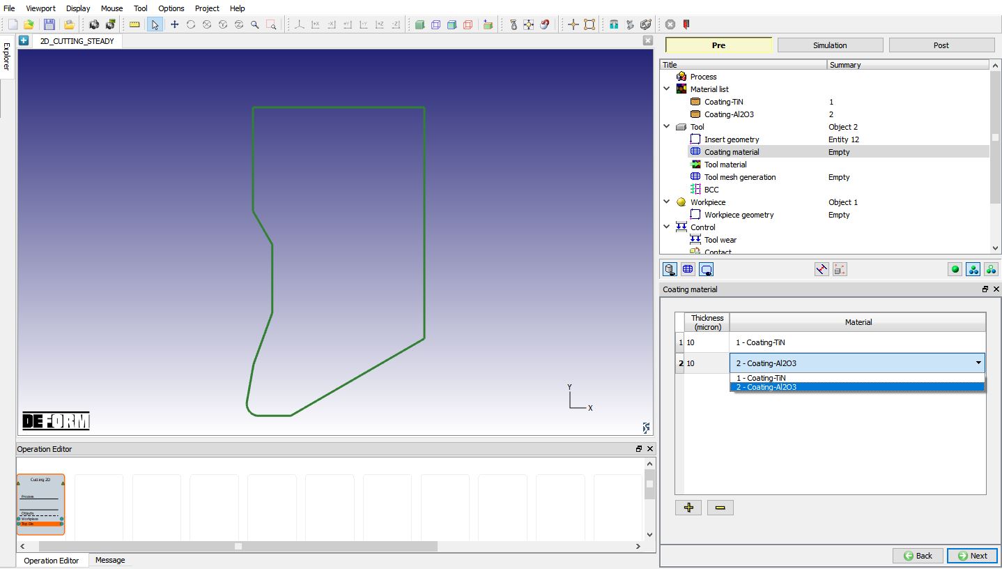
Coating definition

Assign ‘Coating Material’ and thickness in Coating material table, add () two layers of coating. For the outer layer select 10 microns as coating thickness and ‘TiN’ as the material and for the inner layer select 10 microns as the coating thickness and ‘Al2O3’ as the coating layer (see Fig. 2DSSL1.5.). Click on to proceed.

Coating layer and Material Definition

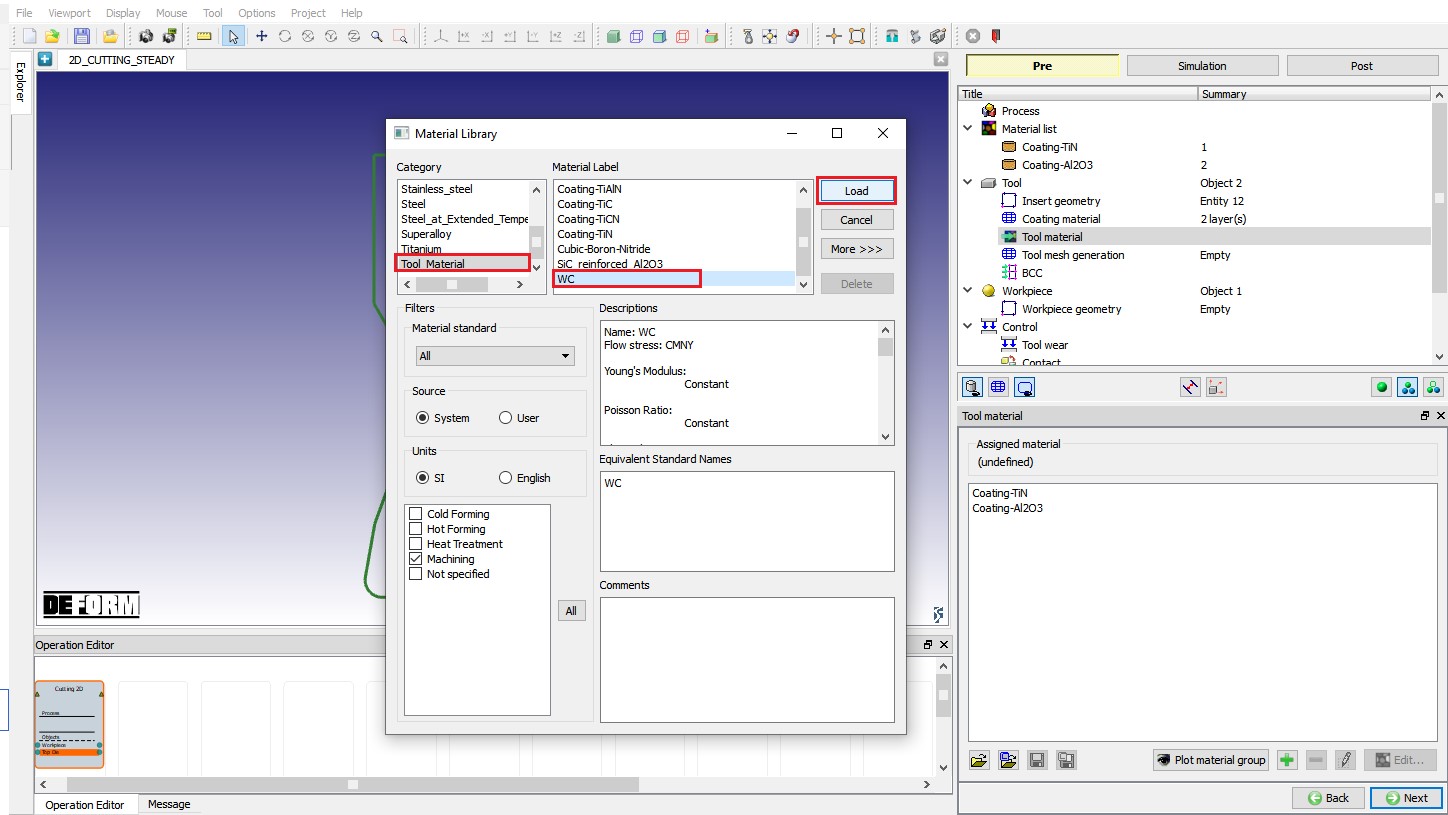
Assign Tool material

In Material Window, click on to Load material data from Library and load ‘WC ‘ material from ‘Tool_Material ‘ category by clicking button as shown in Fig. 2DSSL1.6. Click on to generate Mesh for the Tool.

Loading Tool material from Material Library

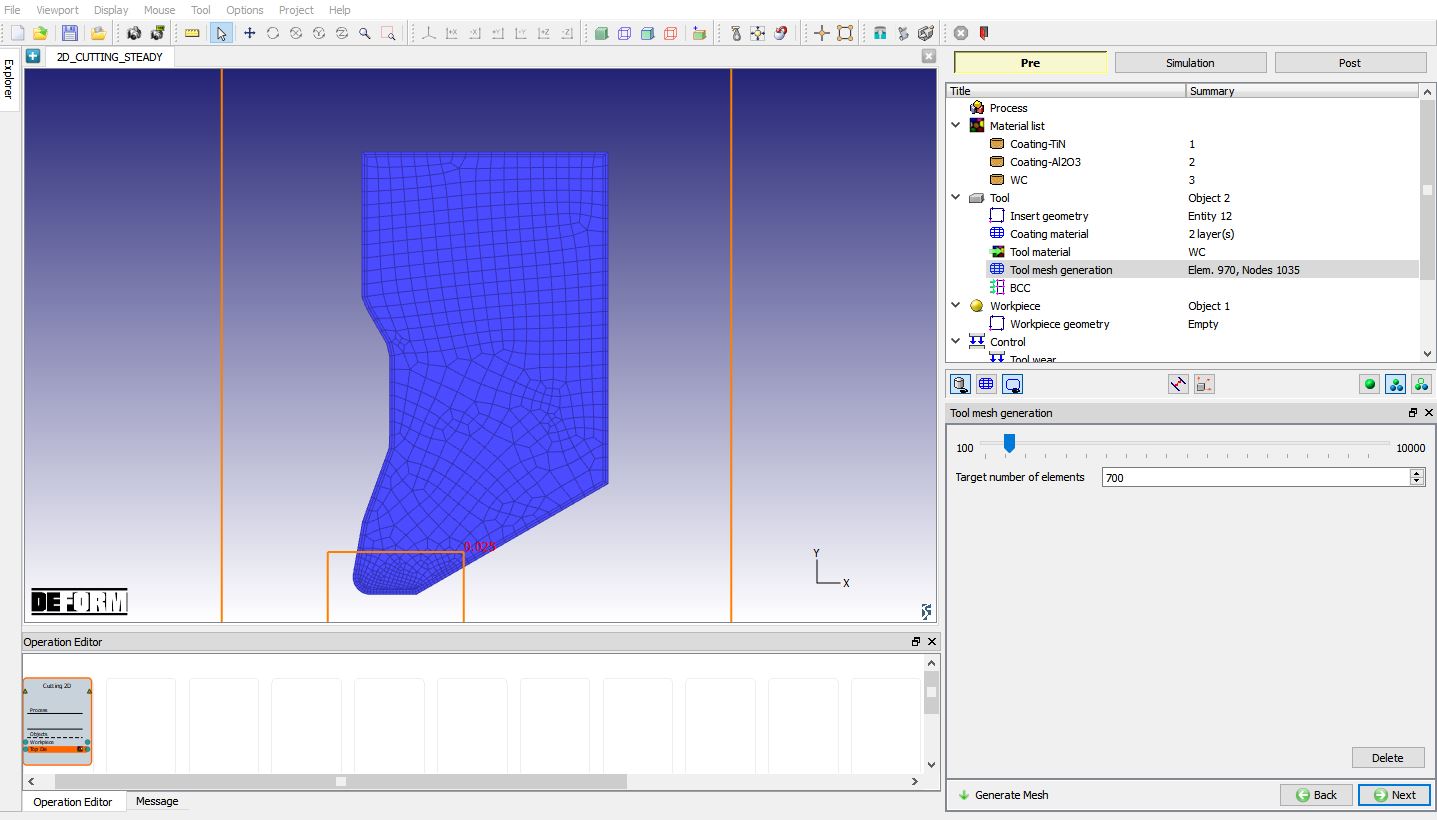
Generating Tool mesh

In the Tool mesh generation menu select ‘700 ’ as the target number of elements for the insert and click on (see Fig. 2DSSL1.7.). Click on to proceed.

Tool Mesh page

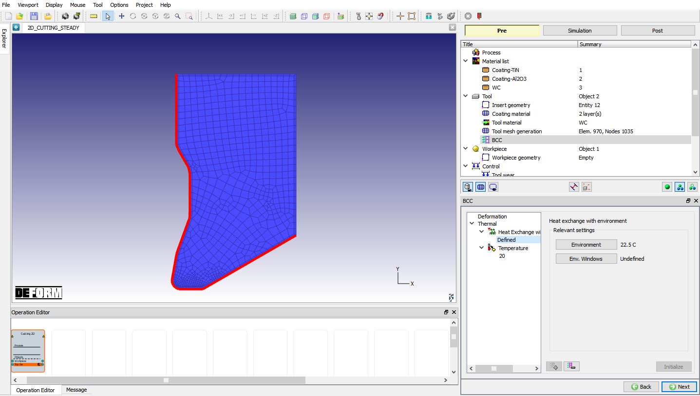
Tool Boundary conditions

Next step is to view the thermal boundary conditions generated by the system in the BCC menu. The program generates heat exchange with environment (part of which comes from insert contact region) and the fixed nodal temperature BCC for the surfaces away from the cutting edge (see Fig. 2DSSL1.8.). Click on to proceed to the workpiece setup.

Tool Boundary Condition

Set the Workpiece geometry

In the ‘Workpiece setup’ define workpiece as a plastic object and temperature as 22.5 °C and click on to proceed. Click on label in the ‘Workpiece geometry’ page. Generate geometry using the parameters:

WP length (L) = 4.5, WP height (H) = 1, Cut length(L1) = 1.5, Chip height(H1) = 0.5, Contact length (D) = 0.4, R1 = 0.3, R2 = 0.1, Chip thickness (C1) = 0.165. Click on to create the workpiece geometry (see Fig. 2DSSL1.9.). Click to close this geometry menu and click on to go to Material page.

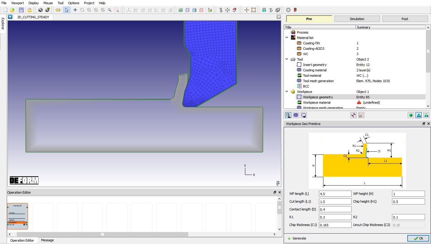
Defining Workpiece geometry

Assigning Workpiece material

In ‘Workpiece material’ page, choose the option ‘import material from library’ option, select ‘Steel ’ category and ‘AISI-1045 (machining) ’, load this material by clicking on button (see Fig. 2DSSL1.10.) and click on to generate Mesh.

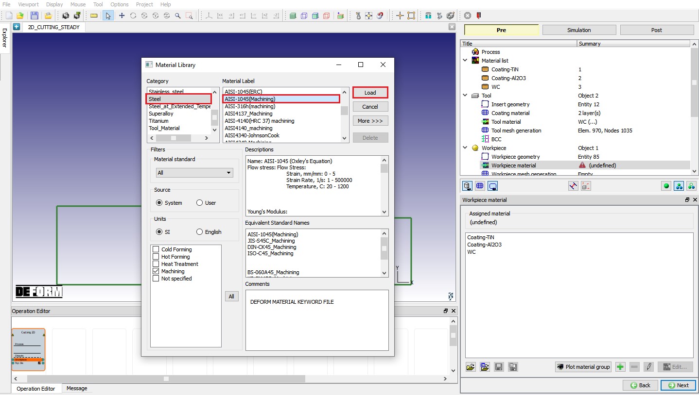
Loading Workpiece material form Library

Generating mesh for Workpiece

Select 15 asNo. of elements through uncut chip thickness for the workpiece and click on to complete mesh generation for the workpiece (see Fig. 2DSSL1.11.). Click on to BCC page.

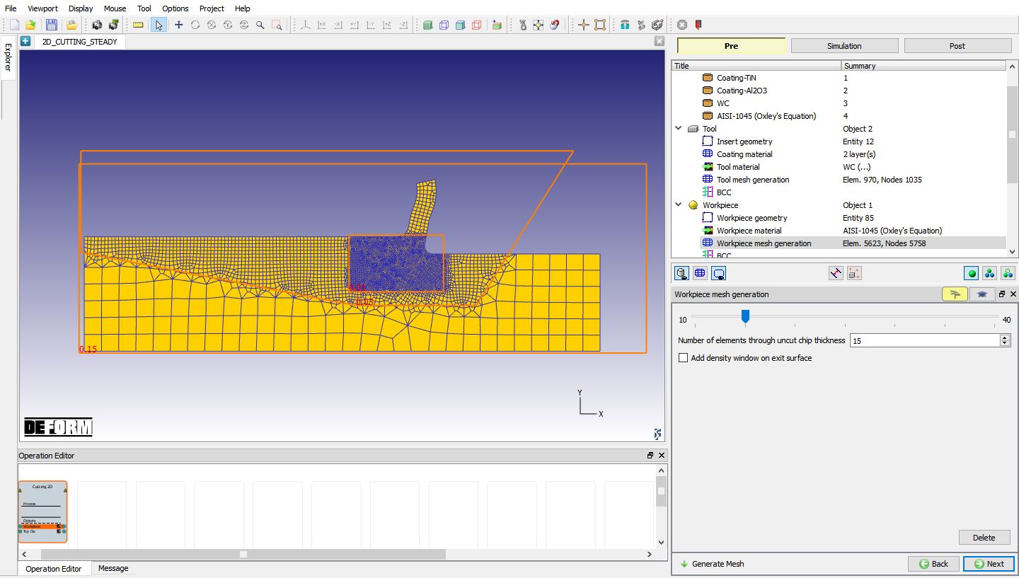
Workpiece mesh page

Workpiece Boundary condition

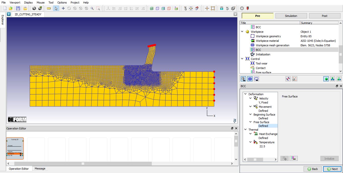
In the ‘View Workpiece BCC’ menu, check the boundary conditions imposed on workpiece by the system (see Fig. 2DSSL1.12.), and click on . Note the velocity BCC assigned to the bottom edge away from the cutting surface to prevent workpiece from flying. From V13.0.1, instead of Surface Velocity (Vx) BCC, Movement BCC will be defined to +X edge and bottom edge of the Workpiece (See Fig. 2DSSL1.12. ) and movement will be defined in Movement page of the Workpiece.

Beginning surface BCC is assigned to the surface (-X edge (left side) of the Workpiece) away from the cutting direction. Free surface BCC is assigned to top edge of the chip and to the surface from where Cutting is started (+X edge (right side) of the Workpiece), See Fig. 2DSSL1.13.

Heat Exchange with BCC is assigned to top edge surface except top edge of the chip. Temperature BCC is assigned +X edge (right side) and bottom edge of the Workpiece, See Fig. 2DSSL1.14. Click on .

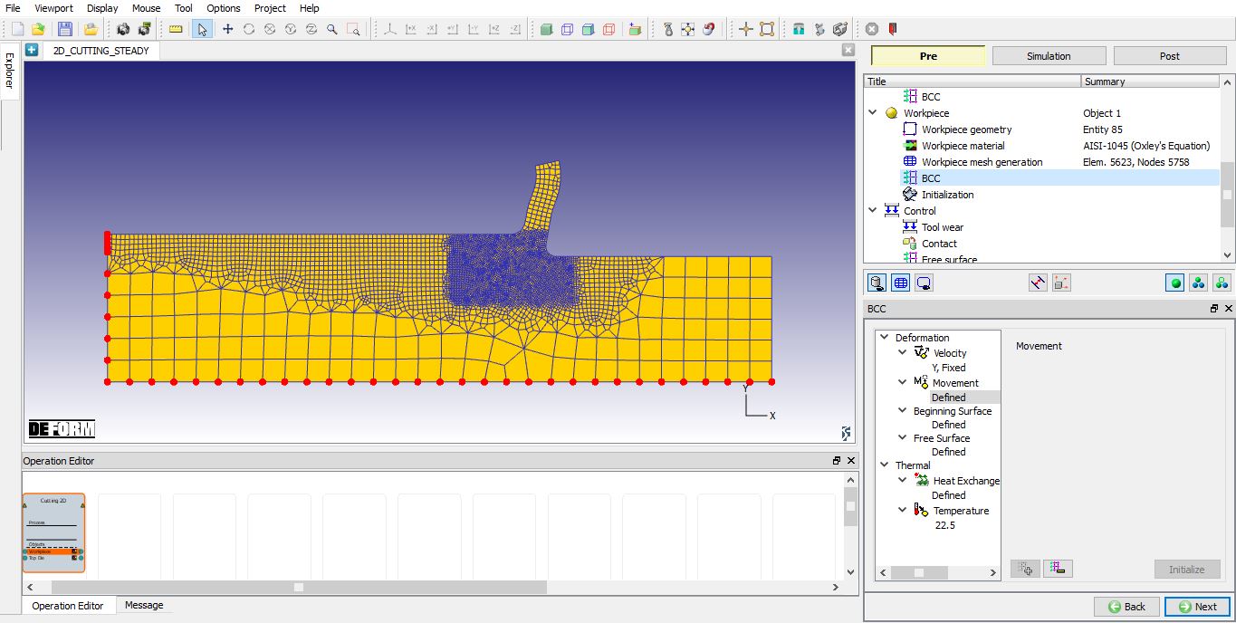
Movement Boundary Condition for Workpiece

Free Surface BCC assigned for Workpiece

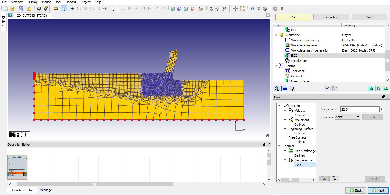
Temperature BCC assigned for Workpiece

Initialization

In Initialize page, we can initialize the workpiece strain value (see Fig. 2DSSL1.15.). In this lab, we are not initializing any strain value, so click on until Tool wear page.

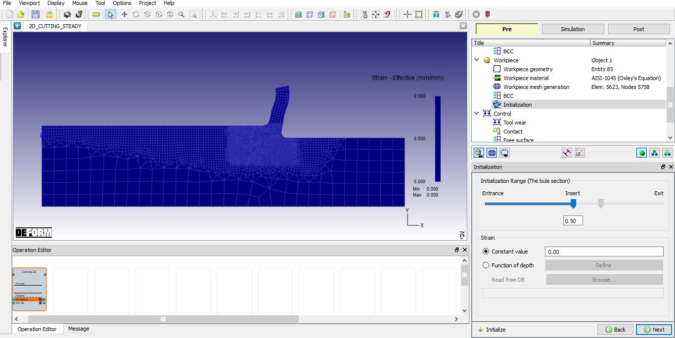
Initialize page

Tool wear setting

Select Usui’s model and input coefficients a, b, please note that these (shown next to the equation) are only some typical values that can be obtained from the literature, and user is responsible for accuracy of this data (see Fig. 2DSSL1.16.). Click on to contact page.

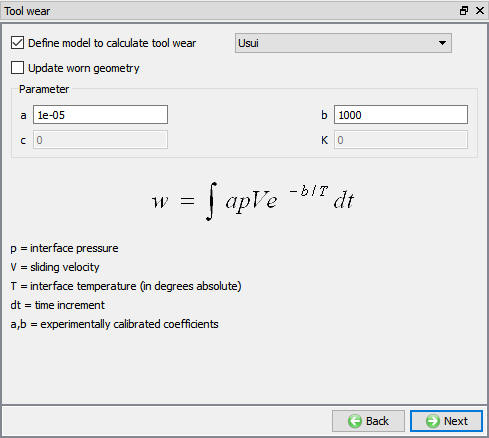
Tool wear setup window

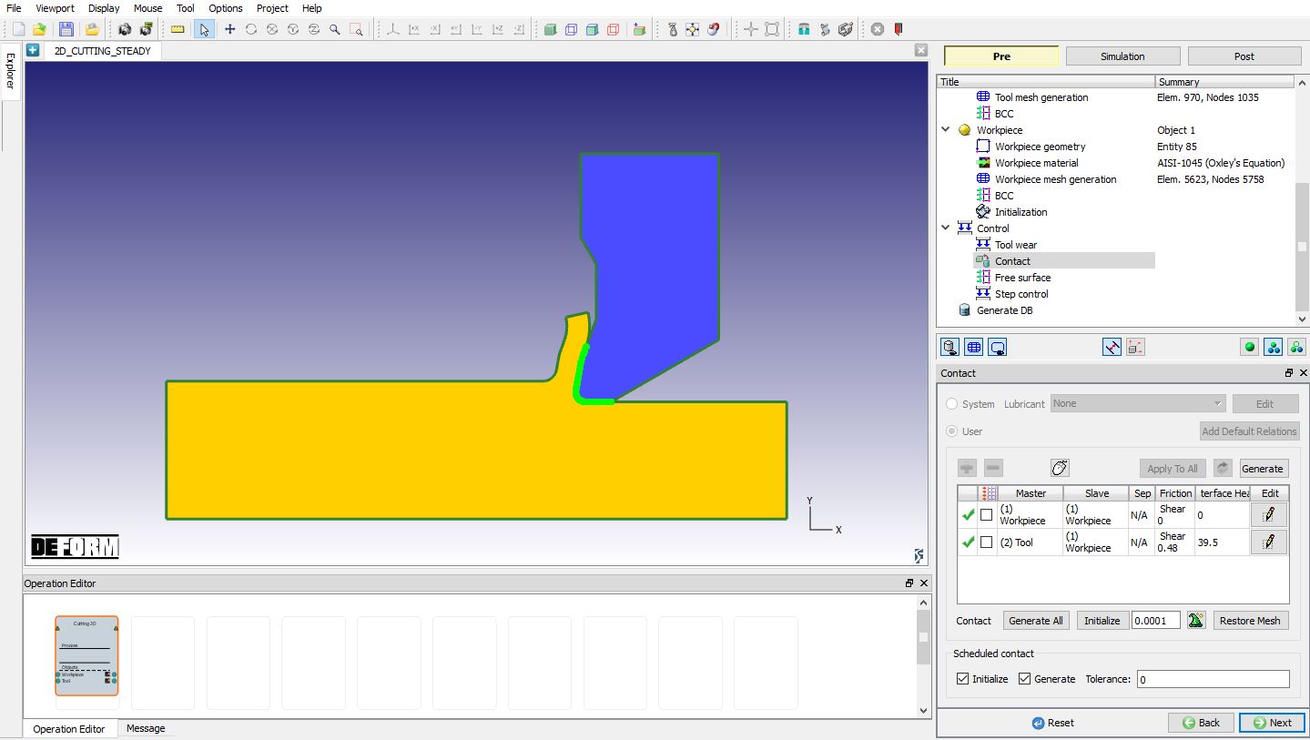
Contact page

In Contact page, use default relations. Click on Tool - Workpiece relation Edit button and define shearfrictionfactor as 0.48 and the interfaceheat transfercoefficient as 39.5N/sec/mm/C , click on to generate contact (as shown in Fig. 2DSSL1.17.). Click on unit Step control page.

Contact page

Step control page

In Step controls page, we will use default Temperature convergence and Strain convergence method which is UL solution: 50 along with default convergence tolerance value (as shown in Fig. 2DSSL1.18.). Click on .

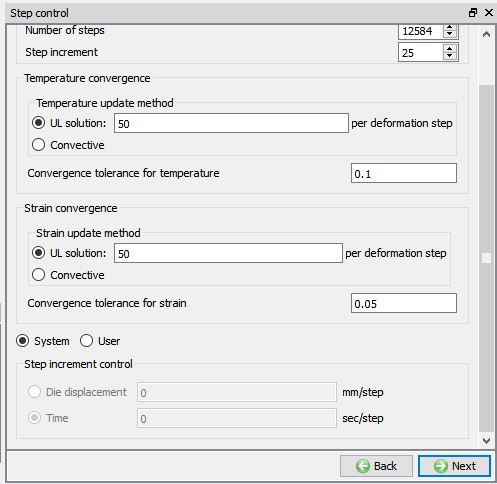
Step Control page

Generate Database

In Generate DB page. Click on the button to generate the database. Observe the message in Message tab informing database generation status.

Running Simulation

Once the database has been generated switch to the Simulation mode by clicking on button above the operation tree. Click on the action label to open the Run Options dialog as shown in Fig. 2DSSL1.19. Use the default ContinueRun option to select “Continue from the last step ” (from step -1) option and then select the Simulation mode as Interactive radio button. Click on button to run the simulation.

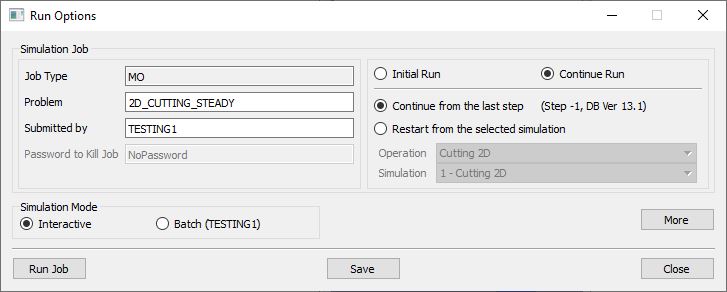
Run Simulation window

Monitor the progress of the simulation by looking at the Simulation Message and Simulation Log tab, making sure that the option is checked. User can view the cutting process as the simulation proceeds to the specified cutting length from Simulation graphics.

When the simulation is finished by reaching steady state, we can observe that the following message is added to the end of the Message file:

Steady state thermal solution has converged

Steady state strain solution has converged

Steady state chip free surface computations have converged

**Message***

Steady state solution has converged

Post Processing

When the simulation is completed, review the results by switching to Post mode using the button above the Simulation tool bar.

Plot Temperature State variable, play through the steps and look the temperature generated in Cutting zone (see Fig. 2DSSL1.20.) .

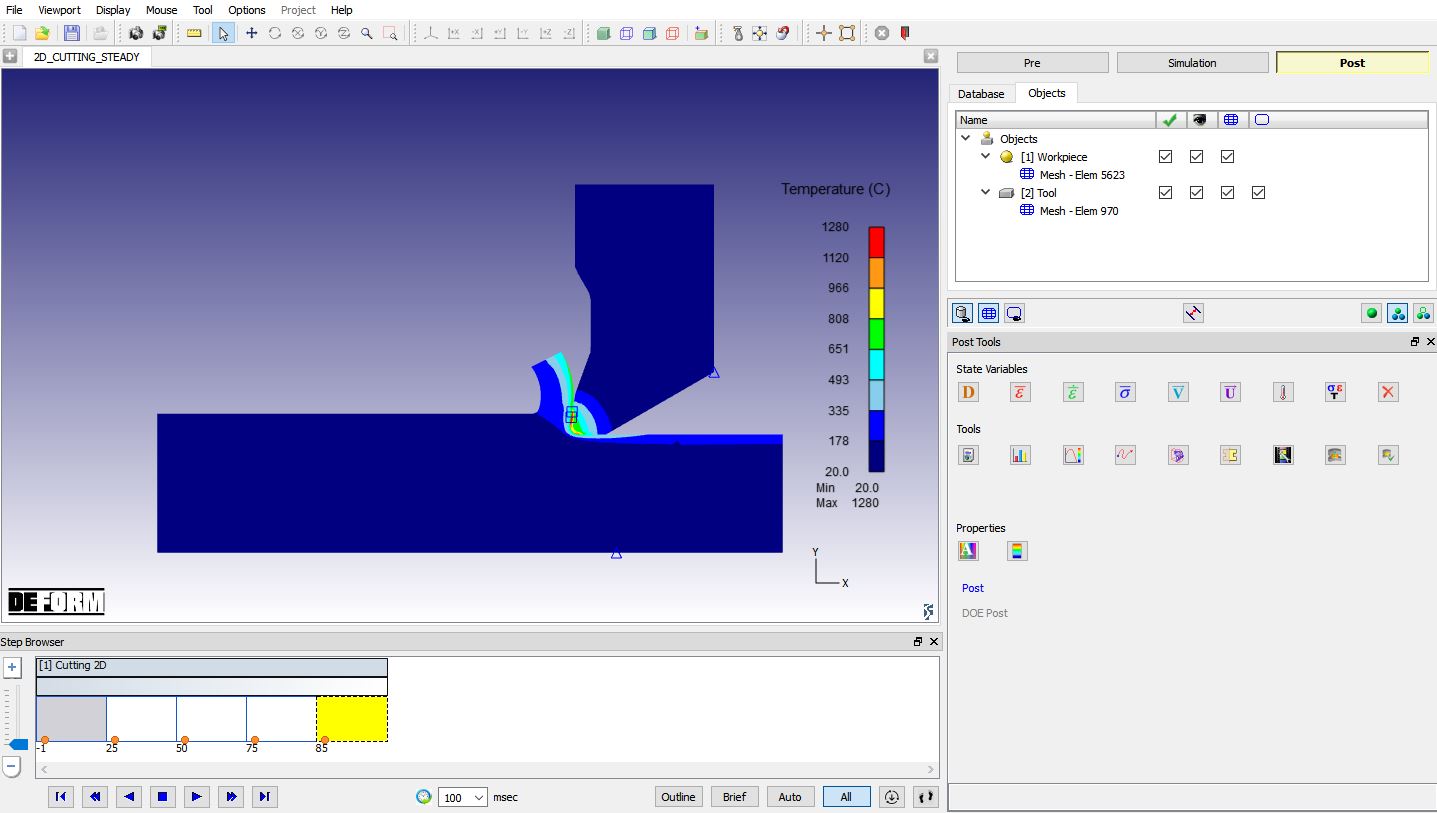
Temperature plot in Steady state Cutting operation

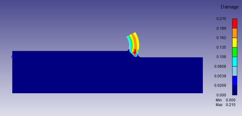
Damage plot for workpiece object