53.1. Optimization Setup

53.1.1. Adding Optimization Study

53.1.2. Defining DOE Variables

53.1.3. Failed DOE Variable definition

53.1.4. Deleting DOE Variable

53.1.5. DOE Table

53.1.6. Defining Case variables

53.1.7. Deleting Case variable

53.1.8. Case variable table

53.1.9. Case definition table

53.1.10. Defining Shape optimization operation

53.1.10.1. Operation selection

53.1.10.2. Define Outputs

Defining Region of Interest

Probe

Operation min/max value

Local min/max Value (Summary min/max (One step))

State variable in regions (State Variable min/max (One step))

Summary plot (all steps from selected operation)

Probe output

53.1.10.3. Define Variable constraints

53.1.10.4. Define Fill constraints

53.1.10.5. Global Min/Max (All steps)

53.1.10.6. Define Objective Function

53.1.10.7. Define Optimization controls

53.1.10.8. Define Stopping controls

53.1.10.9. Database Management

Adding Optimization Study

User must have nominal setup to which Optimization Study can be added. Optimization Study can be added either before completion of nominal simulation or without completion of nominal simulation from V12, while in previous versions Optimization Study can be added only after completion of the nominal simulation. User can add Optimization operation using Add Optimization Study option from (Add new study) button as shown in Fig. 53.1.1.

Adding Optimization Study Project

After adding the Optimization study, Optimization study project gets added next to the nominal project and adds Shape Optimization output operation automatically for adding variables to study in DOE post as shown in Fig. 53.1.2.

Optimization Project with Shape Optimization operation

Defining DOE Variables

The material properties, object data, inter-object data and process variables can be added as DOE variables from property editor window. In Property editor window, if a variable field has green ribbon around the fields (See Fig. 53.1.3.) then that variable can be added as DOE or Case variable. Constants, functions and geometry data definition types can also be added as DOE variables. The DOE variable can be continuous or discrete.

Continuous Input Variable : Continuous variables can be added as normal DOE variable by defining the range of study variables fluctuation/uncertainty as upper and lower bound values and number of samples required within the range. Example object temperature etc.

Discrete Input Variable : Variables which are not continuous can be defined as discrete DOE variables by defining number of samples and sample values. Example billet diameter etc. DOE variable can also be named by the user.

Steps to define DOE Variable

The steps to define the DOE variables are as follows,

1. Before adding the DOE variable user needs to select the operation for which DOE variable needs to be defined. (See Fig. 53.1.2.)

2. Identify the variables to add as DOE variables, fields which are having green ribbon around them in property editor window can only be selected. Right click in green ribbon region and select Add DOE variable option as shown in Fig. 53.1.3.

Adding DOE variable by right click on green ribbon of Study variable field

1. In DOE variable definition window, if DOE variable is continuous then define study variable range as upper and lower bound values as shown in Fig. 53.1.4. else if data is not continuous, define the discrete samples by checking the Discrete checkbox and selecting number of samples to input as shown in Fig. 53.1.5. The default number of samples are three, user can increase the number of samples as required.

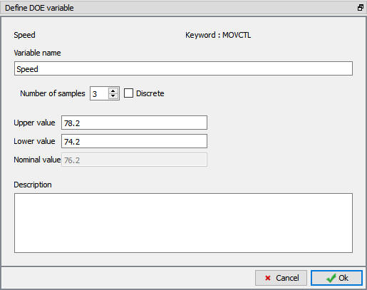
Study variable definition window for Die Speed constant value

Discrete DOE variable definition window for constant value data

1. Enter description for the DOE variable if necessary, as shown in Fig. 53.1.4. Some useful note about the selection and variation defined can be entered here. Click to close the definition.

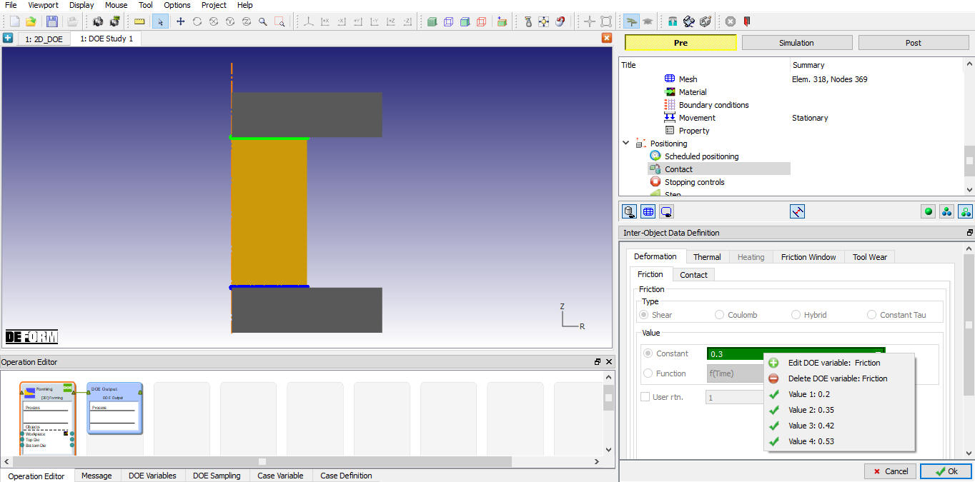
2. Confirm the DOE variable definition by observing the green fill around the variable field after definition. The field filled with green color indicates that it has been added as DOE variable. Right click in the green colored area will display the defined upper and lower bound values (See Fig. 53.1.6. and Fig. 53.1.7.).

DOE variable definition indicators

Discrete DOE variable definition indicators

In operation editor green color DOE text can be observed on operations top right end indicating operations with DOE variables are defined as shown in Fig. 53.1.6. and Fig. 53.1.7. DOE variable name can be edited from “DOE Variables” tab.

The examples mentioned below demonstrates adding different input data types as DOE variable.

Example1: Material property like flow stress, which is function of strain, strain rate and temperature can be added as DOE variable by offsetting or scaling the function curve. Files required to exercise this example are available at installation path 3D\LABS\Gear_blank, open the Gear_blank.moprj file from , simulate the Nominal run and add Optimization study and follow instructions as mentioned below. First add the DOE variable by navigating to material page and using right click option on Flow stress (Define) button as shown in Fig. 53.1.8.

Add function data as DOE variable

In DOE definition window, add description about definition and click on button to define continuous DOE definition upper and lower bound values as shown in Fig. 53.1.9. or if you need to experiment with specific flow stress data of different materials, select discrete DOE definition by checking “Discrete” checkbox and select as many samples as needed to input as shown in Fig. 53.1.10. For Discrete samples definition, click on the button under edit column to define flow stress curves. We will use continuous DOE variable for this example.

DOE variable definition window for function value data Flow stress

Discrete DOE variable definition window for function value data Flow stress

Function definition window will open with nominal values when we click on button for Continuous DOE as shown in Fig. 53.1.11. or button for discrete DOE definition as shown in Fig. 53.1.12. For function data of continuous DOE variable definition, user can select definition type such as Nominal, Upper or Lower from DOE field pull down menu. User can only change the Upper and Lower bound curves using scale, offset options or by editing values or by dragging the curve or point.

For function data of discrete DOE variable, user can define the sample value using scale, offset options or by editing values or importing the flow stress curves DAT file as shown in Fig. 53.1.12.

Nominal function data curves

Nominal function data curves of Flow Stress for Discrete DOE

Select the DOE type as Upper to define the upper bound values. Values can be defined by using scale or offset options. In this example we will define it by scaling the function data. Select Scale radio button and enter 1.01 to scale up nominal stress curves by 1%. Click on Set to apply. See Fig. 53.1.13. for scaled upper bound curves.

Upper bound scaled up function curves

Select the DOE type as Lower to define the lower bound values by using scale option. Select Scale radio button and enter 0.99 to scale down nominal stress curves by 1%. Click on Set to apply. See Fig. 53.1.14. for scaled down lower bound curves.

Lower bound scaled down function curves

Confirm the definition by observing the green fill in define button and green color Optimization text in operation editor on operation right top corner. Right click in the green colored area and confirm whether upper and lower bound values are defined (See Fig. 53.1.15.).

Study variable right click options

Example2 : Object geometry can be added as normal DOE variable using 2d geometry editor or using discrete DOE definition by directly importing different geometry designs. Continuous DOE definition is done by varying the nominal geometry values to define the upper and lower bound geometries. Files required to exercise this example are available at installation path 3D\LABS\Gear_blank. Open the Gear_blank.moprj file from then simulate the Nominal run and add Optimization study. Follow below description to complete Optimization study setup. (To exercise 2D geometry adding as Study variable refer Defining DOE variables- Example2).

First to add the workpiece geometry as Study variable, navigate to geometry page of workpiece and right click on button next to variable field as shown in Fig. 53.1.16.

Geometry variation adding as DOE variable

Add description and click on button (See Fig. 53.1.17.) to define upper and lower bound geometry profiles.

Geometry Study variable definition window

The 3d Geo tool window will open with morphing wizard window to guide user to add upper and lower boundaries as shown in Fig. 53.1.18.

3D Geo Tool window with Morphing wizard

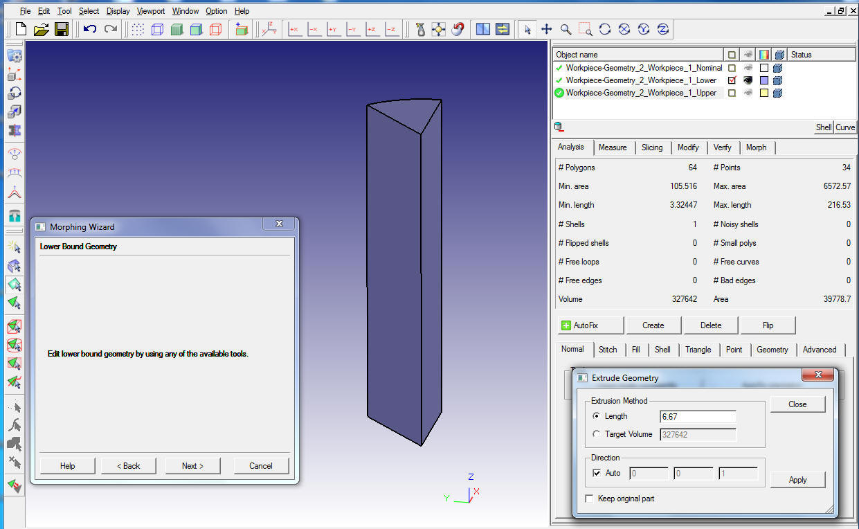
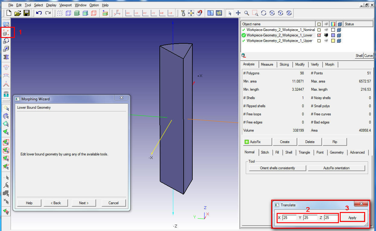
Click to Morphing wizard to open the Lower bound geometry window, edit the geometry using available tools to define the lower bound geometry. In this example geometry height is reduced from 207.01 to 200.64, we will be using (Offset) option for this, so select the offset icon and pick the top face to offset to 6.37 in -Z direction by entering -6.37. Click to perform the offset. as shown in Fig. 53.1.19.

Reducing the object height by Offset option

Observe the lower bound geometry after offsetting as shown in Fig. 53.1.20.

Object Height after offset

Select (Scale) option to scale only the diameter of the cylinder as shown in Fig. 53.1.21., check only X and Y direction check box to scale only diameter not height, enter the scaling factor 1.05748 as shown in Fig. 53.1.22. Click button to perform scaling.

Selecting the scale window to scale cylinder object diameter

After scaling the cylinder object diameter

After defining the lower bound geometry click button to complete Lower bound Morphing. User needs to select the reference plane for the nominal and lower bound geometries, using Pick curve option select Top edges of Nominal geometry and Lower geometry and click on Add button to add connect pair data in table (as shown in Fig. 53.1.23.).

Added connectivity between nominal and lower bound geometries

Similarly select Bottom edges of Nominal geometry and Lower geometry and click on Add button. Then click on Calculate button in Morph tab to build the connectivity between nominal and lower bound geometries as shown in Fig. 53.1.24.

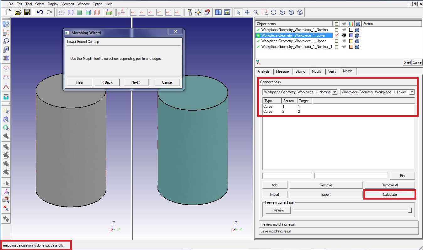
Added connectivity between nominal and lower bound geometries

Click button to define the upper bound geometry. Similar to the lower bound geometry in this example increase the height from 207.01 to 213.68 by offsetting the top face to 6.67 mm and diameter is reduced to 62.5 from 63.5 by scaling factor 0.98425. as shown in Fig. 53.1.25. and Fig. 53.1.26.

Offset geometry height for upper bound geometry

Scaled geometry diameter for upper bound geometry

After defining the upper bound geometry click button to complete Upper bound Morphing, similar to lower bound Morphing, using Pick curve option select Top edges of Nominal geometry and Upper geometry and click on Add button to add connect pair data in table (as shown in Fig. 53.1.27.).

Added connectivity between nominal and upper bound geometries

Similarly select Bottom edges of Nominal geometry and Upper geometry and click on Add button. Then click on Calculate button in Morph tab build the connectivity between nominal and Upper bound geometries as shown in Fig. 53.1.28.

Added connectivity between nominal and Upper bound geometries

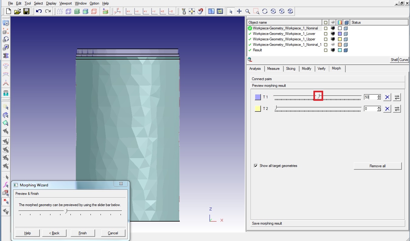
Click button to Preview and Finish page, Morphed geometry can be previewed by selecting the “Preview morphing result” option below connect pairs in Morph tab as shown in Fig. 53.1.29. and Fig. 53.1.30. and sliding the slider bar T1 and T2 for Lower bound and Upper bound respectively.

Morphed geometry between lower bound and nominal

Morphed geometry between upper bound and nominal

It can also be observed from Morphing wizard Preview and Finish window as shown in Fig. 53.1.31. and click on button to close the geometry variable definition.

Morphed geometry from Morphing Preview and Finish window

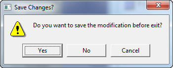
Select Yes to Save Changes popup to save the modification before exiting the 3D Geo Tool, selecting No will not save changes made and cancel will keep the 3D Geo tool will open so that any further changes can be made. (See Fig. 53.1.32.)

Save geometry variable definition popup

Other 3D Geo tool basic tools to define the lower and upper bound geometry are Extrude, Mirror, Rotate and Translate object. These options are briefly described below.

**Extrude **: To extrude an object select the icon then it will popup the extrude geometry popup window as shown in Fig. 53.1.33. In the extrude window select the extrusion length and direction and enter the extrusion length. Click button to extrude the object.

Extrude object window

Checking the Direction auto checkbox will automatically detect the extrusion direction as shown in Fig. 53.1.34.

Object after extrusion in Z direction

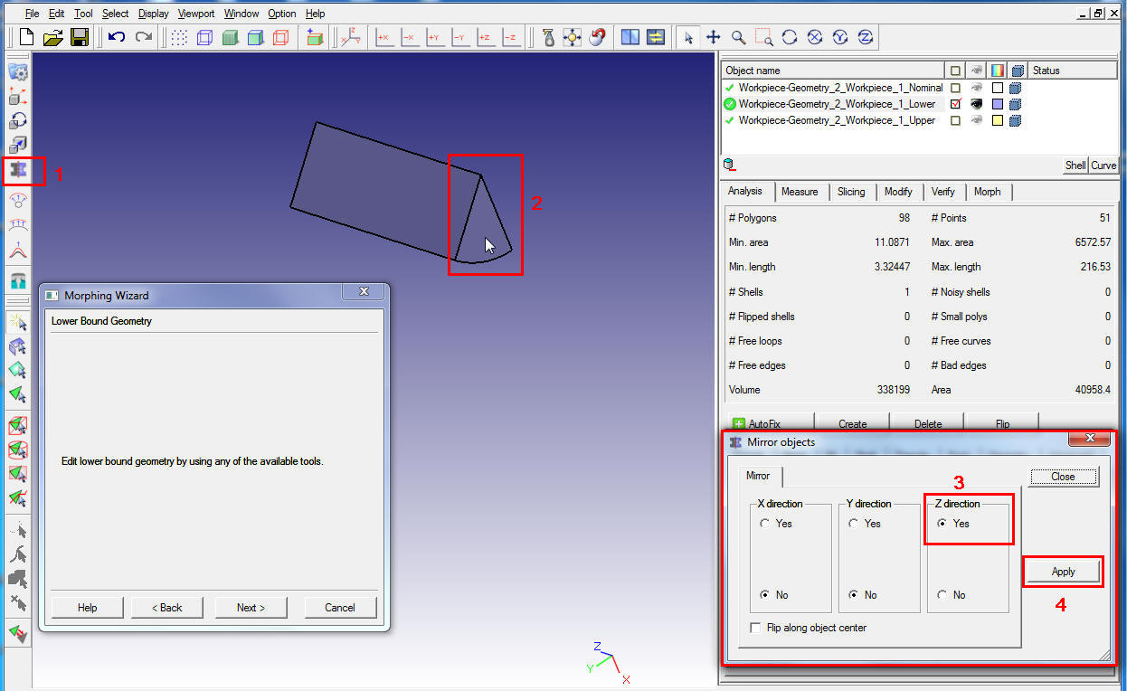
Mirror Object : To mirror an object select icon then it pops up an Mirror Objects window as shown in Fig. 53.1.35. In the Mirror objects window, select Yes for the direction in which object to be mirrored and then click on button to mirror the object.

Mirror Object window

Observe the object after mirroring about Z plane as shown in Fig. 53.1.36.

Object after mirror in Z direction

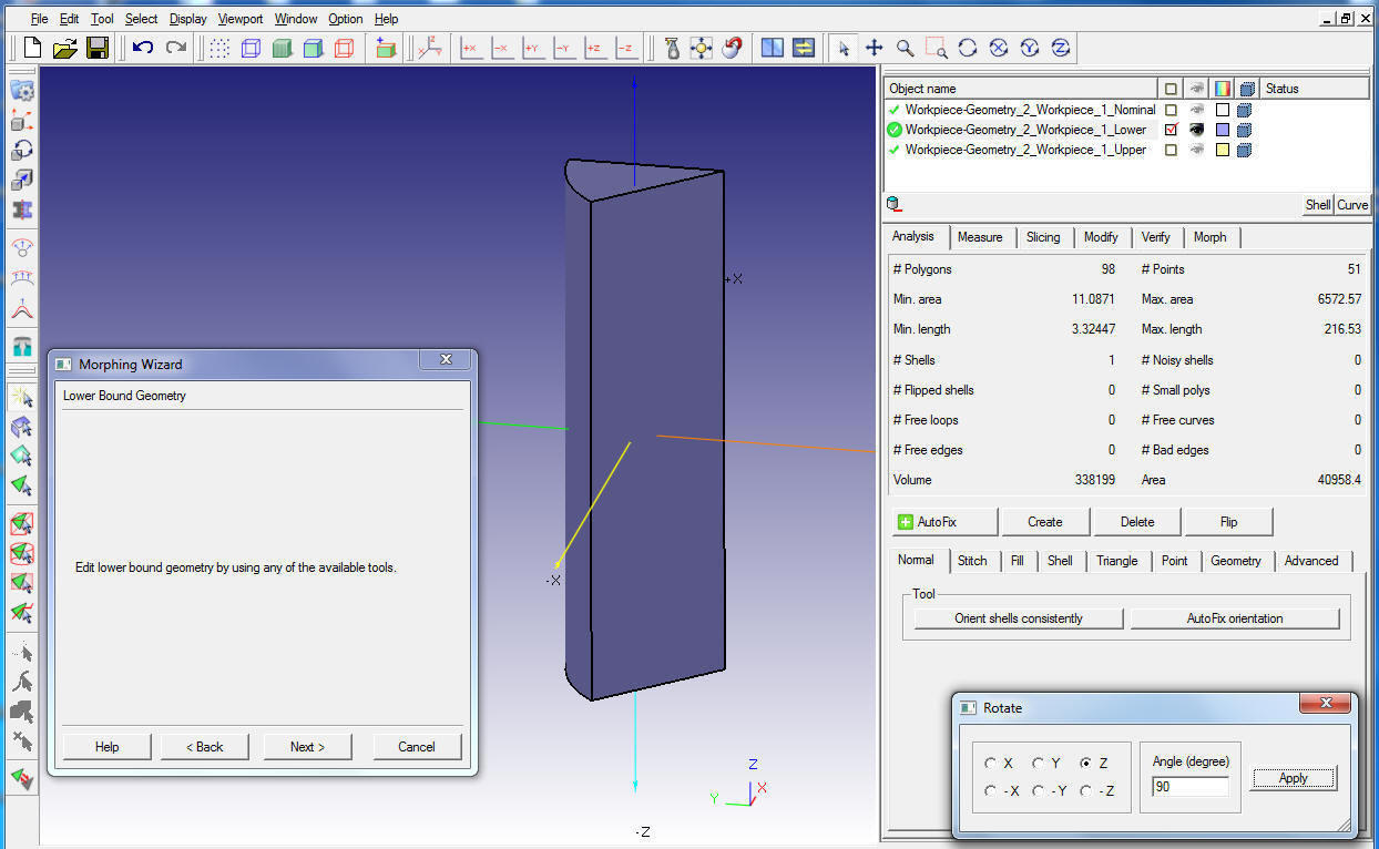
Rotate Object : To rotate an object select icon then it pops up an Rotate window as shown in Fig. 53.1.37. In rotate window select direction about which to rotate and angle, then click on button to rotate the object.

Rotate Object window

Observe the object rotated about 90 deg in Z direction as shown in Fig. 53.1.38.

Object after rotation in Z direction

Translate object : To move object only along X, Y and Z direction select icon then it pops up an Translate window as shown in Fig. 53.1.39. In translate window enter the distance to move about any of three principle directions and then click on button to move the object.

Translate object window

Observe the object after moving in all X, Y and Z direction as shown in Fig. 53.1.40.

Object after moving in X,Y and Z direction

Failed DOE Variable definition

In Optimization design variable definition if upper or lower or both range values are not defined or in discrete DOE definition any discrete samples are not defined then such design variable will be highlighted with red color fill around the field or button as shown in Fig. 53.1.41. Then by right clicking on the field, missing data can be edited and corrected.

Failed DOE variable definition

Deleting DOE Variable

Defined DOE variables will be highlighted by green color shading around DOE variables field (See Fig. 53.1.42.), right click on the defined DOE variable field gives an option to delete the added variable. User can also delete the added DOE variables from DOE table using button or using right mouse button menu option on variables listed in study variable column. (See Fig. 53.1.42.).

Delete Study variable definition

DOE Table

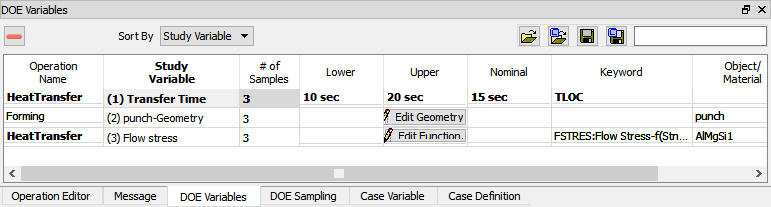
DOE table tabulates the details of DOE variables defined for each operation as shown in Fig. 53.1.43. DOE table includes the details of Operation Name, Study variable (Defined DOE variable) Name, Number of samples, Lower, Upper and Nominal values, Keyword and object or material to which it belongs. User can edit the defined Study variable name, # of samples, constant Lower and Upper bound values for continuous DOE definitions by double clicking on that cell. User can click on in table to edit function data of continuous DOE definition which will open the function DOE definition window. To edit the geometry user can click on in DOE table, which will open 2D geometry editor or 3D geo tool.

For Discrete DOE definition only DOE variable name can be edited directly in table. For constant and function type discrete DOE variable, user must click on in table in the respective variable row then discrete DOE definition window will be opened to edit the values.

DOE table with added DOE study variables details

DOE table terminology:

**Operation Name** : Operation in which DOE Study variable is added.

Study Variable : Name of the Study variable added for DOE study, by default this name is defined by system based on variable selection and can be renamed by the user.

# of Samples : Number of study variable samples to prepare total DOE samplings to study. The number of samples will affect the sampling and the number of simulation studies to be carried over.

Lower : Lower bound value of the study variable in case of continuous DOE variables (for Continuous DOE definition).

Upper : Upper bound value of the study variable in case of continuous DOE variables (for Continuous DOE definition).

Nominal : Nominal value of the study variable in case of continuous DOE variables (for Continuous DOE definition), the values of DOE variables defined in nominal project are considered as nominal values.

Keyword : Keyword which define the added study variable.

Object/Material : It displays the object name to which study variable belongs to or it displays the material name if it belongs to any material properties. In case of process data like heat transfer time system does not display any name.

Delete Study variable : User can select added study variable and delete it using this button.

Export DOE Table : The DOE study variables definition can be saved to an XML file using this option.

Export DOE table to library : This saves the DOE study variables definition to a XML file in user data library. In windows system with user name “user1” the default library path will be “C:\Users\user1\Documents\userDataLib\DOE”.

Import DOE Table : Saved DOE study variable definitions XML file can be imported to redefine the same.

Import DOE Table from library : Saved DOE study variable definitions XML file can be imported from user library to redefine the same.

Sort by: Sort by is used to sort the DOE table display content by operation or by study variables definition order.

DOE table details sorted by study variable number

Link To : DOE Variables can be linked to each other from the right click menu of the selected variable as shown in the Fig. 53.1.45. If DOE variables behavior is similar, then those DOE variables can be linked so that they vary similarly and number of DOE variables for sampling can be reduced. When two variables are linked, in effect they act as single variable and variables for DOE sampling are reduced.

Linking the two different DOE Variables

Defining Case variables

The case variable can be defined for all the fields having green ribbon around them (See Fig. 53.1.46..). Constants, functions and geometry data definition types can be added as case variables. The case variables can only be discrete. Once a case variable is defined then user can observe that the field will be filled with blue color.

Defining a case variable is similar to discrete DOE variable definition hence please refer Discrete Input variable to know about defining case variable definition. Below example demonstrates the case variable definition.

Example1: Material property like flow stress which is function of strain, strain rate and temperature can be added as Case variable by offsetting or scaling the function curve. To exercise this example, required files are available at installation path 3D\LABS\Gear_blank, open the Gear_blank.moprj file from . Simulate the Nominal run, add Optimization study and follow instructions as mentioned below.

First add the Case variable by navigating to Workpiece object page and then using right click option on object temperature field select the Add case variable option as shown in Fig. 53.1.46.

Adding case variable for object temp.

When we click on “Add case variable” option we will get the Define DOE Variable window and we can observe that only discrete type input can be defined. By default, we will be having the 3 samples as shown in the Fig. 53.1.47.

Case variable definition window for object temp. data

We are defining the 3 samples in this example. We must define the samples data from the lower value to upper value as shown in the Fig. 53.1.48. After defining the case variable data click on ok button.

After defining the case variables data

Confirm the definition by observing the Blue fill in “Object temp.” field. Right click in the blue coloured area and confirm the definition of sample data. (See Fig. 53.1.49.)

Right click options after defining the case variable

Deleting Case variable

Defined case variables will be highlighted by blue color shading around variables field (See Fig. 53.1.50.), right click on the defined variable field gives an option to delete the added case variable. User can also delete the added case variables from “Case variables” table using button or right mouse button menu option on variables listed in study variable column (See Fig. 53.1.51.).

Deleting the Case variable

Deleting the case variable from case variable table

Case variable table

Case variable table tabulates the details of case variables defined for each operation as shown in Fig. 53.1.52. Case variable table includes the details of Operation Name, Study variable (Defined Case variable) Name, Number of samples, Lower, Upper and Nominal values, Keyword and object or material to which it belongs. User can edit the defined Study variable name, # of samples, constant Lower and Upper bound values. For Case variable definition only Study variable name can be edited directly in table, while for constant and function data DOE variable user must click on in table in the respective variable row, this will open the discrete DOE definition window.

Case variable table

Case definition table

User can either use full factorial or user defined methods as sampling methods for case variables. (See Fig. 53.1.53.)

Case definition table

Full factorial samples

User defined samples

Defining Shape optimization operation

The Shape optimization operation objective is to define pre-defined required state variables that need to be studied to automatically post-process multiple databases.

Operation selection

Select the Shape optimization operation from operation editor after defining DOE and Case variables to define variables and other settings for post-processing DOE studies.

OPT Output for single operation

OPT output for multi operations

Operation selection page displays all the operations that are defined in the nominal setup and user can select any one operation (See Fig. 53.1.56.) or multiple operations (See Fig. 53.1.57.) by selecting the respective check box and click to define the output for the respective operation. For each operation we can define the Region of Interest, Probes, Output variables, Variable constraints and Fill constraints.

Define Outputs

Once operations for which we are going to define outputs are selected then they are listed in the tree as shown in Fig. 53.1.57. User can select the operation to define outputs, then user can observe output types in property editor window and user need to check the output types for that operation, the selected outputs are added to tree as shown in Fig. 53.1.58. The output types available are Single output, Transient output and Special output types as shown in Fig. 53.1.58.

OPT outputs selection window

Defining Region of Interest:
A Region of Interest (ROI) is a region of an object that could be smaller or larger than the entire object and is used to limit the study to what happens inside the final shape of the part (i.e., machined shape or chip shape). It can be used to study an area to include or exclude for forming feature/defect (end effects, under-fill or fold) and to determine success or failure for the process. (See Fig. 53.1.59.) Multiple ROI can be added from v11.0 onwards in optimization.

Under-fill and unwanted area example

Common mesh is one way of defining the ROI. In common mesh all the results of individual DOE’s are interpolated onto a common mesh for the purpose of comparison and response surface generation. (See Fig. 53.1.60.)

Common mesh concept

To define the ROI region geometry first click on button (See Fig. 53.1.61.) then click on to create ROI using geometry primitives or import the ROI geometry. After creating the ROI geometry other geometry options like Scale, Check, Reverse and object positioning are activated as shown in Fig. 53.1.62.

ROI Definition window for 3D

ROI can be deleted by using the (Delete ROI) button after selecting the respective ROI as shown in Fig. 53.1.62.

After creating ROI geometry for 3D

Probe:
Probe can be used to obtain the co-ordinate data of the point on the object nearest to the probe position, this option would be helpful to validate the geometry of the object. Multiple probes with different probe types and orientation can be defined.

To add a probe and define its data like shape, orientation and position, click on button in the Probe page (See Fig. 53.1.63.),

1. Select Probe Shape from Type pull down menu,

2. Define the Probe size in Size field.

3. Define the orientation of the probe in Approach Direction field,

4. Define Start position Coordinate of the Probe and

5. Click next toprobe output page to define the outputs.

Probe definition window

Operation min/max value:
Selected state variable minimum / maximum value is plotted across all steps and all simulations of the selected operation for the selected object.
To select the state variable first click on button to add rows and double click on each cell under Variable row to select state variable and double click on the cell in the same row under components to select the maximum or minimum or other directional components and Min/Max to select options like Min., Max., (Absolute)Min., (Absolute)Max., Diff (Max and Min difference), Average and Standard Deviation based on requirement. In Fig. 53.1.64. out of minimum Temperature values of all steps Max. value and out of maximum Effective strain state values of all steps Max. value for workpiece and Top die Z-Load Absolute Max. values are added as output variables across all steps of the operation.

Operation Min/Max state variable for all step’s selection window

Local min/max Value (Summary min/max (One step)):
Selected state variable output’s minimum / maximum value is plotted at last step of selected operation for the selected object.

To select the state variable first click on button to add rows and double click on each cell under variable row to select state variable and double click on the cell in the same row under components to select the maximum or minimum or directional components based on requirement. In Fig. 53.1.65. Maximum Effective strain and Effective stress state variables for workpiece object and Top die Z-Load variables are added as Local min/max output of the operation.

Summary Min/Max state variable for one step selection window

State variable in regions (State Variable min/max (One step)):
Selected state variable component output’s min/max and other computed value is plotted at last step of selected operation for the selected object, region of interest or probe.
To select the state variable first click on button to add rows and double click on each cell under Variable row to select state variable and double click on the cells in the same row to select component, Min/Max, Object and Region/Probe under respective columns. For State variable output type, components will be the variable components like Directional values or Effective or Principal, Mean etc. Min/Max will give options like Min., Max., (Absolute)Min., (Absolute)Max., Diff (Max and Min difference), Average and Standard Deviation. In Fig. 53.1.66. Maximum Effective stress of whole workpiece object, Maximum Effective strain within the region defined and Maximum Damage within probe are added.

State variable Min/Max within a region for one step selection window

Summary plot (all steps from selected operation):
The selected state variables summary throughout all the steps of the selected operation is plotted.

Add state variables using button and select X-axis, state variable, components and object. In Fig. 53.1.67. we have select the Maximum effective strain with respect to time for workpiece, Minimum temperature with respect to time for workpiece and Z-Load with respect to stroke for Top die.

Summary plot selection window

Probe output:
Probe output can be used to obtain the co-ordinate data of the point on the object nearest to the probe position, this option would be helpful to validate the geometry of the object. Multiple probes with different probe types and orientation can be defined. (See Fig. 53.1.68.)

Probe output selection window

Define Variable constraints

Variables Constraints can define constraints by selecting the respective variables from the left side of the window and clicking on the button to add constraint and constraint value as shown in Fig. 53.1.69. The constraint can be Less than, Greater than or Min-Max difference Less than depending on the variable. Constraints can be applied to object or any Region available in pull down menu as shown in Fig. 53.1.70. Constraints can be removed by selecting the added constraint from right side window list and clicking on the button.

Variable constraints definition window

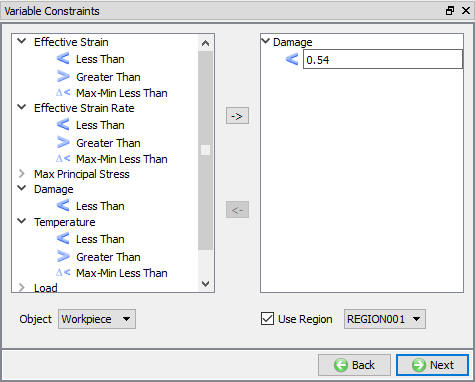
Variable constraint for ROI

Define Fill constraints

In Fill constraints window user can check the fill constraints like Complete Fill, Under fill volume ratio, Minimum die distance and No Fold constraint.

Complete Fill : Complete Fill constraint will check the die fill, user can also select the interested region to check the die fill using ROI.

Underfill volume ratio: Run cases can be constrained as pass/fail based on underfill volume ratio compared with specified percentage value.

Minimum die distance : Run cases can also be constrained as pass/fail based on surface nodes distance and comparing with specified value.

No folds : No folds option is used to check the run without fold in selected object or region and constrained as fail if there is a fold.

These constraints checks are tabulated as Pass/Fail in DOE post table for easy analysis (See Fig. 53.1.71.)

Fill constraints Definition Window

Global Min/Max (All steps)

Selected state variable minimum / maximum value is plotted across all steps of all operations for the selected object.

To select the state variable first click on button to add rows and double click on each cell under Variable row to select state variable and double click on the cell in the same row under components to select the maximum or minimum or other directional components and MIn/Max to select options like Min., Max., (Absolute)Min., (Absolute)Max., Diff (Max and Min difference), Average and Standard Deviation based on requirement. In Fig. 53.1.72. out of minimum Temperature values of all steps Max. value and out of maximum Effective strain state values of all steps Max. value for workpiece and Top die Z-Load Absolute Max. values are added as global min/max outputs.

Global Min/Max state variable for all steps selection window

Define Objective Function

The objective function is used to run optimization process using the defined DOE and Case variables. The Objective function can be defined in three types they are,

1. Single

2. Weighted sum

3. Equation

Single
Objective function has to be define by selecting the state variable and its objective for a particular object, operation and specific region of the object can also be selected (See Fig. 53.1.73.).Different objective options are available depending on variables and, those are Minimize, Maximize, Minimize Min/Max Difference and Minimize error from target value and Minimize error from target curve. Major variables are grouped to ease the definition, apart from major variables other variables are also available to add as objective function in the respective state variable groups. Now all state variables can be added as objective functions for optimization. Only one objective function is allowed per optimization study.

Objective Function window for single type

Weighted Sum
Using the Weighted sum type objective function, we can define the multiple variable by selecting the respective check box and defining the reference value and scale value. The priority of the multi state variables will be depending on the weight value defined. (See Fig. 53.1.74.)

Objective Function window for Weighted Sum type

Equation
Using the Equation type Objective function, the optimization process is defined as equation from the defined output state variables. We can use the function pull down menu to select the operator. (See Fig. 53.1.75.)

Objective Function window for Equation type

Define Optimization controls

The user can select the check box to Enable LHC sampling as shown in the Fig. 53.1.76. The LHC (Latin hypercube) sampling is a statistical method for generating a near-random sample of parameter values from the defined DOE and Case variables. The user can select the LHC up to Level 1, 2 & 3. After selecting the level, we must define the multiplier for that respective level and scope reducer using the slider bar. The total LHC runs will be calculated automatically from the above data. The optimization can be stopped or continued after completion LHC runs based on gradient algorithm.

Optimization control page

Define Stopping controls

Optimization simulation can be stopped by two stopping controls those are Maximum Simulations and If objective function error is less than defined value as shown in Fig. 53.1.77.
When optimization is started initially 8 times of design variables simulations are simulated to set up response surface and continues depending on simultaneous runs defined in run options until stop criterion is met. It will stop when total simulation runs exceeds or equal to the user defined Max simulation number or when error in objective function value is less than the user specified value in Objective function less than field.

Optimization stopping criteria window

Database Management

DOE / Optimization study involves multiple simulations and requires large amount of storage space. User can manage the size of these projects using options available in Database output page. In Database output page, user can select the steps that can be stored in DB by selecting suitable option. If DOE/ Optimization study is already completed and still the user would like to control the storage space then user can select the suitable option in Database output page and click on button. (See Fig. 53.1.78.).

Save Only Last Step in Database : Using this option we can save only Last step data in database.

Save First/Last Step in Database : Using this option we can save only First and Last step data in database.

Save First/Last Step of Each operation in Database : Using this option we can save First and Last step data of Each operation data in database.

Save First/Last Step and Remesh steps in Database : Using this option we can save First step and Last step and Remesh steps data in database.

Save All Step in Database : Using this option we can save data of All Steps in database.

Optimization Database Management window