Spinning Lab
In this Lab we will be setting up simple Spinning process with ALE model and Implicit solver
1.1. Creating a New Problem
1.2. Process Page
1.3. Simulation setup
1.4. Objects
1.5. Workpiece
1.6. Mandrel
1.7. Tail stock
1.8. Roll
1.9. Pass Table
1.10. Controls
1.11. Contact
1.12. Stopping Controls
1.13. Simulation controls
1.14. Generate Database
1.15. Running Simulation
1.16. Post processing
Creating a New Problem
On a Windows machine , go to the ![]() button select DEFORM-v1x.xxx (.xxx indicates version number E.g. v14.0.2) and select DEFORM GUI Main vxx.xx from the menu. The DEFORM GUI Main window will appear.
button select DEFORM-v1x.xxx (.xxx indicates version number E.g. v14.0.2) and select DEFORM GUI Main vxx.xx from the menu. The DEFORM GUI Main window will appear.
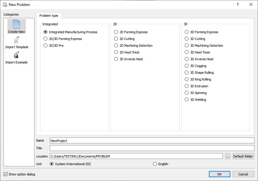
Create a new problem either by selecting File![]() **New Problem** or by clicking the New Problem
**New Problem** or by clicking the New Problem ![]() icon. The Problem Setup window will appear as shown in Fig. 3DSPL1.1. Select “ Integrated Manufacturing Process “ radio button and Unit system as “SI “ using radio button. Define Problem Name as “SpinLab “ and make sure the “Show option dialog” check box is turned on (if we do not turn on the “Show option dialog ” check box, then we will not get the New Project dialog in MO UI). Then click on
icon. The Problem Setup window will appear as shown in Fig. 3DSPL1.1. Select “ Integrated Manufacturing Process “ radio button and Unit system as “SI “ using radio button. Define Problem Name as “SpinLab “ and make sure the “Show option dialog” check box is turned on (if we do not turn on the “Show option dialog ” check box, then we will not get the New Project dialog in MO UI). Then click on ![]() button to open a new Problem using the Deform Integrated Manufacturing Process.
button to open a new Problem using the Deform Integrated Manufacturing Process.
New Problem page
Multiple operation wizard will open with the New Project dialog, At this point user will be prompted to specify a project name (system will create a separate folder with this project name) and title for this session. In this session we will use ‘SpinLab’ as the project name. 3D Spinning operation can also be added in “New Project” dialog, in this lab we will add Spinning g operation from Explorer operation list, so do not check “First operation” check box in “New Project” dialog. Click on ![]() to continue to open the operation.
to continue to open the operation.
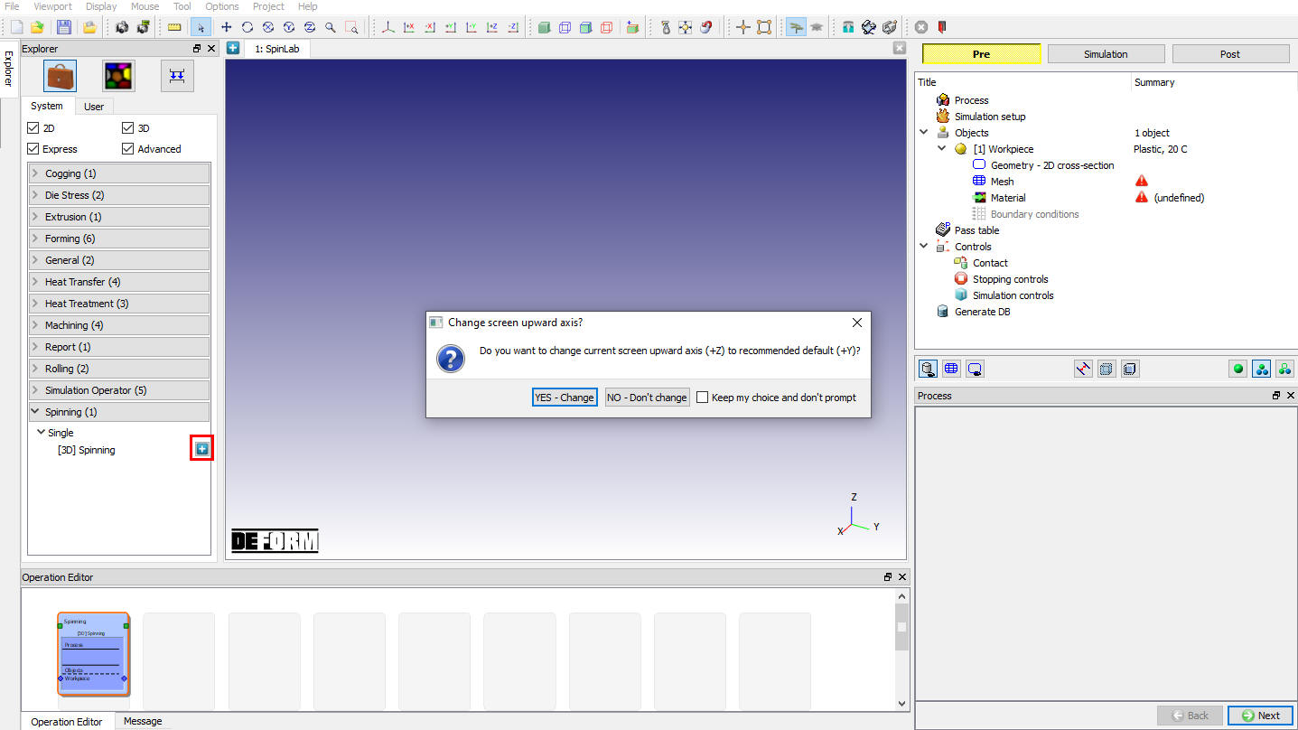
Add 3D Spinning operation from the Explorer Operations list. Add the operation by clicking on ![]() button available next to 3D Spinning or user can also add by drag and drop into the Operation Editor (see Fig. 3DSPL1.2.). When we add the Spinning operation, If the current Screen upward direction is “Z” direction then we will get below popup. Click “YES-Change “ in “Change screen upward axis” popup.
button available next to 3D Spinning or user can also add by drag and drop into the Operation Editor (see Fig. 3DSPL1.2.). When we add the Spinning operation, If the current Screen upward direction is “Z” direction then we will get below popup. Click “YES-Change “ in “Change screen upward axis” popup.
Screen upward direction popup
Now the process settings window will open by default. 3D Spinning operation can also be added from Operation Explorer in MO.
Opened 3D Spinning operation
Process Page
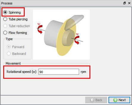
In Process page select “Spinning “ and define Mandrel Rotationalspeed as 90 rpm as shown in Fig. 3DSPL1.4. This speed is also applied to both tail stock and head stock if we used. Click on ![]() to Simulation setup page.
to Simulation setup page.
Process page
Simulation setup
In Simulation setup, select solution method as “ALE “ and solver type as “Implicit “. Since, we are not interested in temperature profile we will select “Constant temperature (isothermal) “ type Thermal calculation and Turn on Active in FEM check box to activate Target volume calculation (see Fig. 3DSPL1.5.). Click on ![]() to Objects page.
to Objects page.
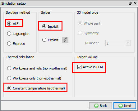
Simulation setup page
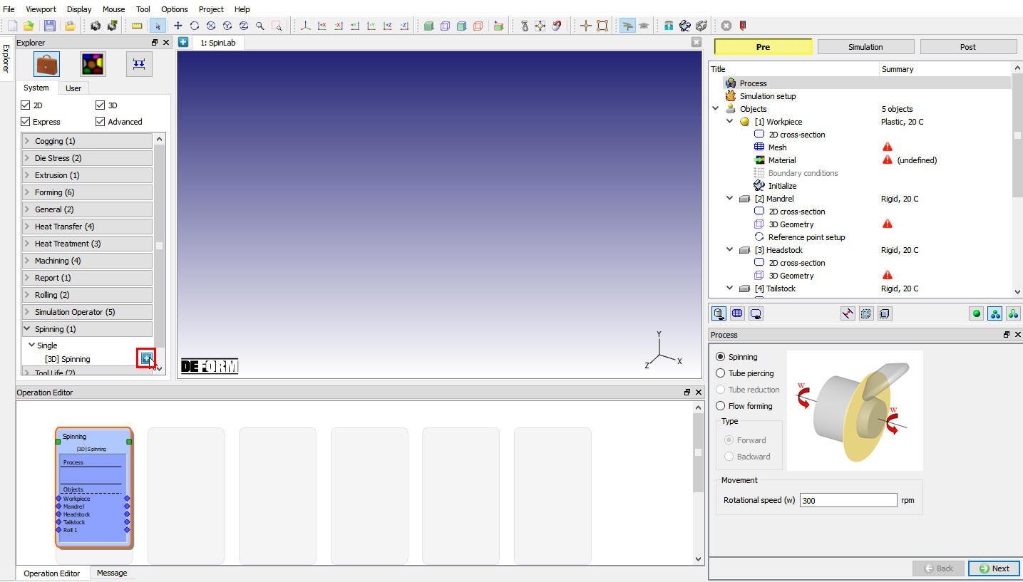
Objects
In this spinning lab, we will use Workpiece, Mandrel, Tail stock and one Roll. In Objects list, by default Mandrel, Tail stock and Head stock check box will be checked. Uncheck the Head stock check box and keep Number of Rolls as 1 as shown in Fig. 3DSPL1.6. Click on ![]() to Workpiece page.
to Workpiece page.
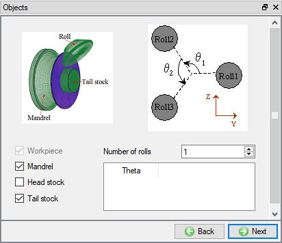
Objects list
Workpiece
In the Workpiece page, keep the object name as Workpiece , object temperature of 20°C and Object type as Plastic as shown in Fig. 3DSPL1.7. Click on ![]() to 2D Geometry page.
to 2D Geometry page.
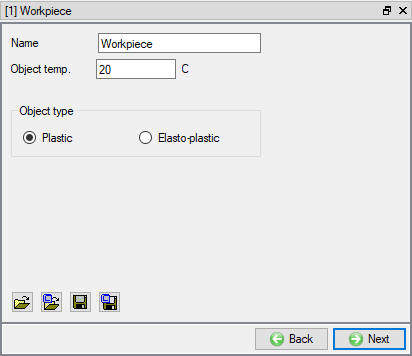
Workpiece General page
Importing Workpiece 2D Geometry
Import 2D geometry, “SpinLab-blank.DXF ” from the “3D/Labs/Spinning” folder. Click on ![]() and then click on Check and correct geometry in the pop-up to verify the geometry. The geometry will be corrected for its orientation, click
and then click on Check and correct geometry in the pop-up to verify the geometry. The geometry will be corrected for its orientation, click ![]() in the message pop-up window and then ok button to close the geometry verification window. Click on
in the message pop-up window and then ok button to close the geometry verification window. Click on ![]() to Mesh page.
to Mesh page.
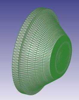
Generating Mesh
In mesh page, select mesh type as Brick mesh and define Target number of Elements as 90 for Cross section mesh. For 3D mesh define Number of revolved sections as 100. Since the set up is ALE implicit we need finer mesh at contact for capturing accurate contact hence, we will define Finer Mesh in the contact region by 15 degree Angle and Size ratio as 4. Click on ![]() and then click on
and then click on ![]() . The mesh should look like as shown in Fig. 3DSPL1.8. Click on
. The mesh should look like as shown in Fig. 3DSPL1.8. Click on ![]() to Material page.
to Material page.
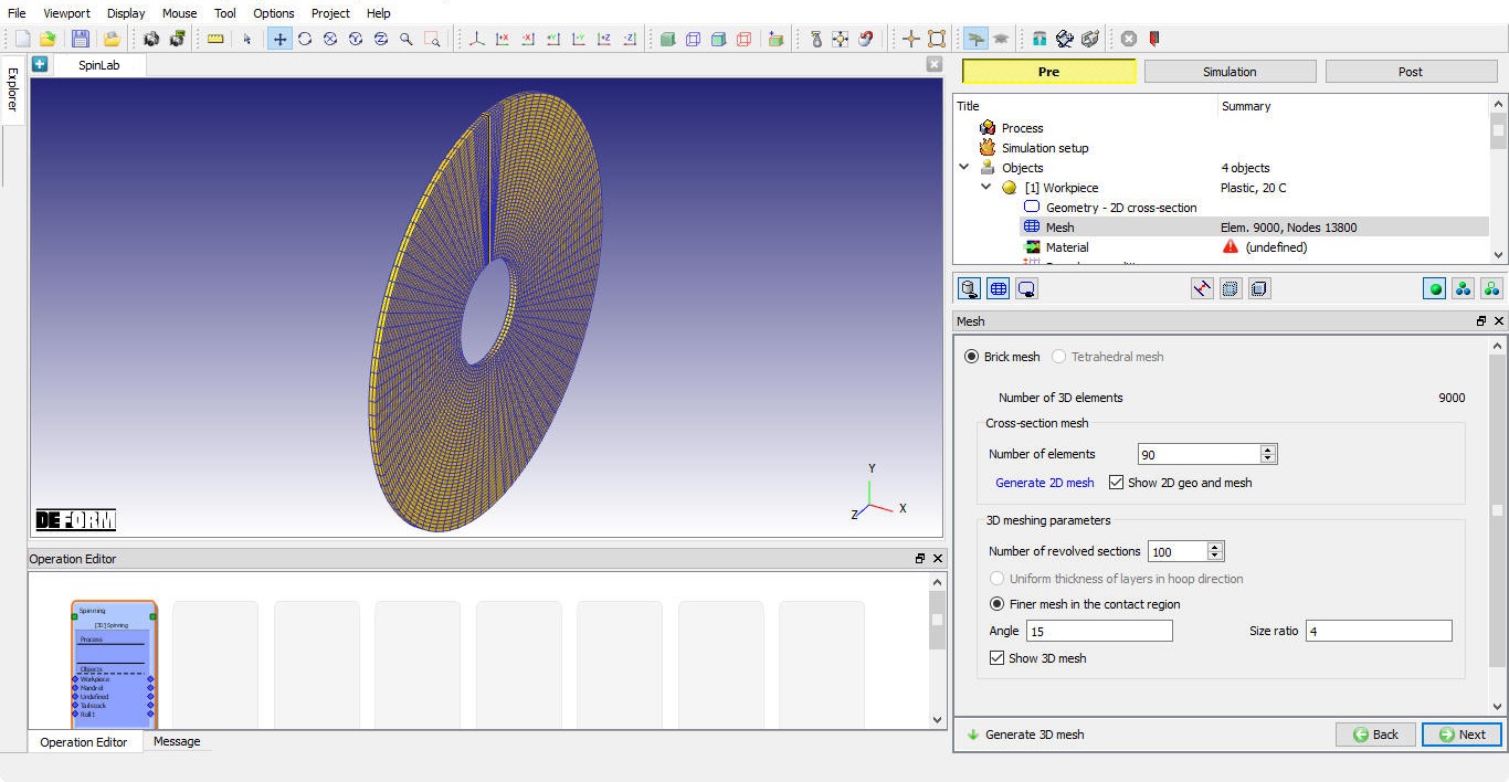
Generated 3D Mesh for Workpiece
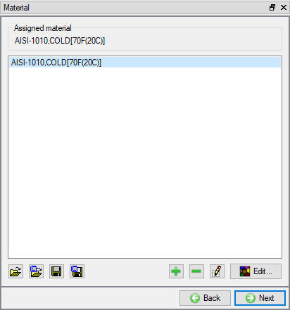
Assign Material
In Material page, click on ![]() (Load material from library) icon and load the material Steel group material “AISI-1010,COLD[70F(20C)] “ from material library window. Assign the “AISI-1010,COLD[70F(20C)] “ material for Workpiece as shown in Fig. 3DSPL1.9. Click on
(Load material from library) icon and load the material Steel group material “AISI-1010,COLD[70F(20C)] “ from material library window. Assign the “AISI-1010,COLD[70F(20C)] “ material for Workpiece as shown in Fig. 3DSPL1.9. Click on ![]() until Mandrel page.
until Mandrel page.
Assigning Material for Workpiece
Mandrel
In the Mandrel General page keep the default values for name as Mandrel and temperature as 200°C. Click on ![]() to Geometry 2D cross-section page.
to Geometry 2D cross-section page.
Importing Mandrel 2D Geometry - Cross section
Import 2D geometry, “SpinLab-mandrel.DXF ” from the “3D/Labs/Spinning” folder. Click on ![]() and then click on Check and correct geometry in the pop-up to verify the geometry. The geometry will be corrected for its orientation, click ok in the message pop-up window and then click
and then click on Check and correct geometry in the pop-up to verify the geometry. The geometry will be corrected for its orientation, click ok in the message pop-up window and then click ![]() button to close the geometry verification window. Click on
button to close the geometry verification window. Click on ![]() to 3D Geometry page.
to 3D Geometry page.
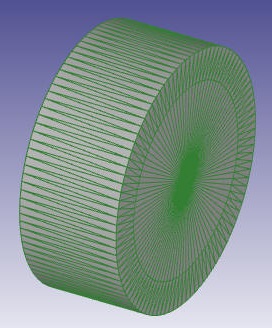
Generate Mandrel 3D Geometry
Using default value of 100 as “Number of revolved sections” generate 3D geometry by clicking on ![]() option (see Fig. 3DSPL1.10.). Click on
option (see Fig. 3DSPL1.10.). Click on ![]() to Reference point setup page.
to Reference point setup page.
Generated Mandrel 3D Geometry
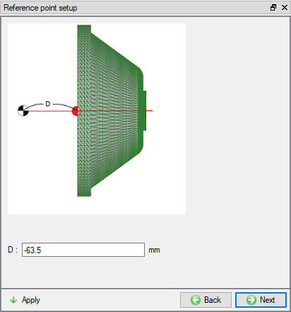
Mandrel Reference Page
In this page we can define Reference point of Mandrel, we will use default calculated value of D “-63.5” as shown in Fig. 3DSPL1.11. “D” is the distance between the Deform Origin and the origin of the Mandrel along X axis and will be used to position the mandrel. Click on ![]() to Tail Stock page.
to Tail Stock page.
Reference point setup page
Tail stock
In the Tail stock General page keep the default values for name as Tail stock and temperature as 200°C. Click on ![]() to Geometry 2D cross- section page.
to Geometry 2D cross- section page.
Importing Tail stock 2D Geometry - Cross section
Import 2D geometry, “SpinLab-tailstock.DXF ” from the “3D/Labs/Spinning “ folder. Click on ![]() and then click on
and then click on ![]() in the pop-up to verify the geometry. The geometry will be corrected for its orientation, click ok in the message pop-up window and then
in the pop-up to verify the geometry. The geometry will be corrected for its orientation, click ok in the message pop-up window and then ![]() button to close the geometry verification window. Click on
button to close the geometry verification window. Click on ![]() to 3D Geometry page.
to 3D Geometry page.
Generate Tail stock 3D Geometry
Using default value of 100 for “Number of revolved sections “ generate 3D geometry by clicking on ![]() option (see Fig. 3DSPL1.12.). Click on
option (see Fig. 3DSPL1.12.). Click on ![]() to Roll page.
to Roll page.
Generated Tail stock 3D geometry
Roll
In the Roll General page keep the default values for name as Roll and temperature as 200°C. Click ![]() to 2D cross- section page.
to 2D cross- section page.
Importing Roll 2D Geometry - Cross section
Import 2D geometry, “SpinLab-roll.DXF ” from the “3D/Labs/Spinning “ folder. Click on ![]() and then click on
and then click on ![]() in the pop-up to verify the geometry. The geometry will be corrected for its orientation, click ok in the message pop-up window and then
in the pop-up to verify the geometry. The geometry will be corrected for its orientation, click ok in the message pop-up window and then ![]() button to close the geometry verification window. Click on
button to close the geometry verification window. Click on ![]() to 3D Geometry page.
to 3D Geometry page.
Generate Roll 3D Geometry
Using default value 100 for “Number of revolved sections “ generate 3D geometry by clicking on ![]() option (see Fig. 3DSPL1.13.). Click on
option (see Fig. 3DSPL1.13.). Click on ![]() to Orientation page.
to Orientation page.
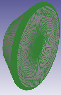
Generated Roll 3D geometry
Orientation
In this lab the movement of the roll along the mandrel axis is defined using path movement which requires roll datum to be defined. It should be noted that rolls require a unique setup approach due to their use of the path movement control. Roll translation will be defined by a path that is applied in a local UV (axial/radial) coordinate system. A single point on the roll, the reference point (datum), will follow this path. The current location of the reference point, and thus the roll, is determined by the path data and the current time. Each roll following a path must have a reference point defined for it.
User can select the Roll datum point using the button ![]() next to Roll Datum field (see Fig. 3DSPL1.15.) which will provide options as shown in Fig. 3DSPL1.16. User can also enter the Datum Co-ordinates manually. In this lab, Rotation center will be selected in Roll Datum wizard dialog, path definition for the roller are already properly configured according to the origin (0,0) reference point hence we will leave Roll Datum co-ordinates to default (0,0).
next to Roll Datum field (see Fig. 3DSPL1.15.) which will provide options as shown in Fig. 3DSPL1.16. User can also enter the Datum Co-ordinates manually. In this lab, Rotation center will be selected in Roll Datum wizard dialog, path definition for the roller are already properly configured according to the origin (0,0) reference point hence we will leave Roll Datum co-ordinates to default (0,0).
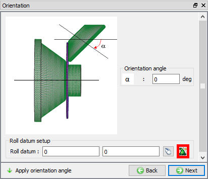
Orientation page
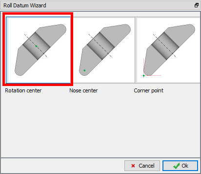
Roll Datum Wizard
The roll needs to be tilted to the proper spinning orientation, which is 45 degrees in this case. To do so, in Orientation page define Orientation angle as 45 as shown in Fig. 3DSPL1.16. and click ![]() . Click on
. Click on ![]() to Pass Table page.
to Pass Table page.
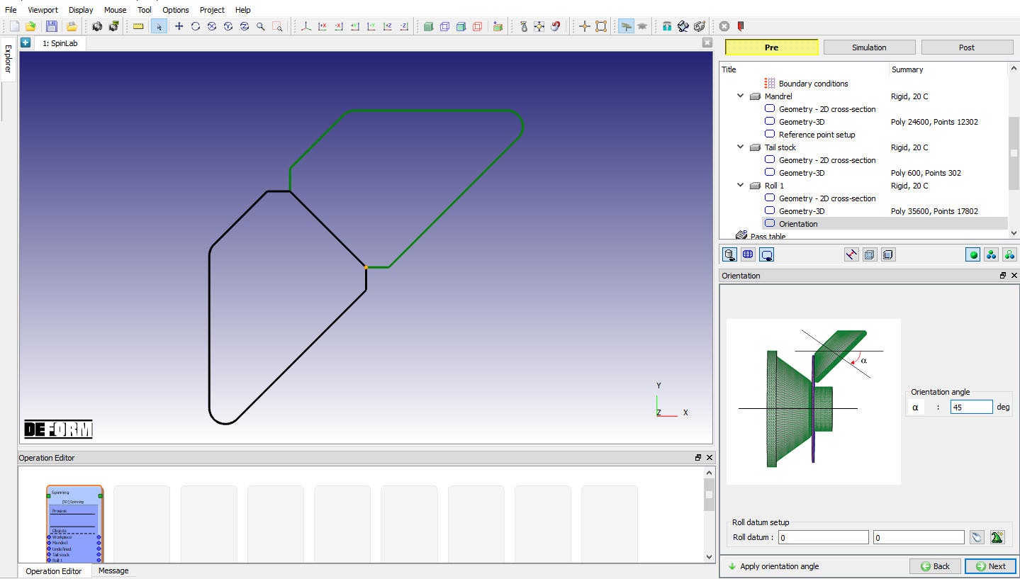
Roll Orientation page
Pass Table
Click on ![]() button to define Movement for Roll 1 in Pass table (see Fig. 3DSPL1.17.).
button to define Movement for Roll 1 in Pass table (see Fig. 3DSPL1.17.).
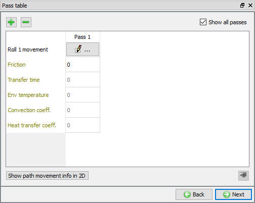
Path Table window
Since the roll moves along a particular path we will select Path and definition of path type as Function of Time path type as shown in Fig. 3DSPL1.18.
Note that curvilinear G-Code path data must be reduced to linear data, since DEFORM does not support curvilinear paths.
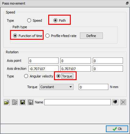
Roll 1 Movement page
Click ![]() and click
and click ![]() to open SpinLab-roll-path_table.dat. from/3D/Labs/Spinning folder. Change the plot type to U-V to see a graphical representation of the axial (U) and radial (V) roller movement profile (see Fig. 3DSPL1.20.). Click
to open SpinLab-roll-path_table.dat. from/3D/Labs/Spinning folder. Change the plot type to U-V to see a graphical representation of the axial (U) and radial (V) roller movement profile (see Fig. 3DSPL1.20.). Click ![]() in Synchronization with path movement popup and click
in Synchronization with path movement popup and click ![]() to close the definition.
to close the definition.
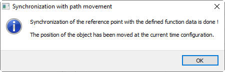
Synchronization with path movement popup
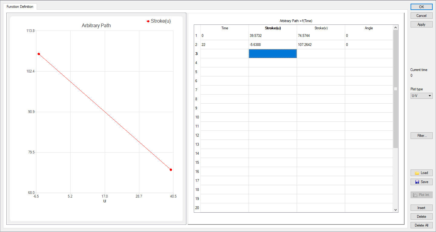
U-V Plot
Note that the Rotation 1 center point is already defined by the path translation data.
Select Rotation type as “Torque “ for Roll 1and leave the value at 0 since the roll rotates based on torque free. Click on ![]() to close movement page. We will not define any other values for this lab and click on
to close movement page. We will not define any other values for this lab and click on ![]() to Positioning page.
to Positioning page.
Controls
All of the objects that are mounted along the machine axis (headstock, mandrel, workpiece, tailstock) were imported at the correct location.
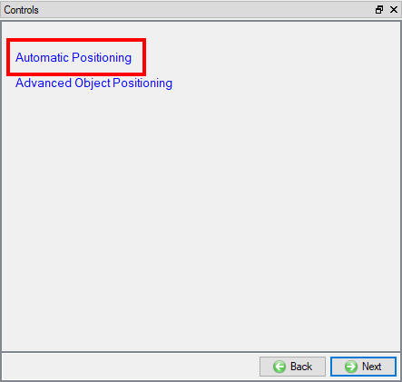
Automatic positioning issue
Go to Controls page, then click on Automatic Positioning. Initial (t=0) option will move the roller to the path location of time = 0. At contact option will move the roller to the path location of the time at contact. Use At contact and click on ![]() . Click
. Click ![]() in popup. Click on
in popup. Click on ![]() to close Contact page.
to close Contact page.
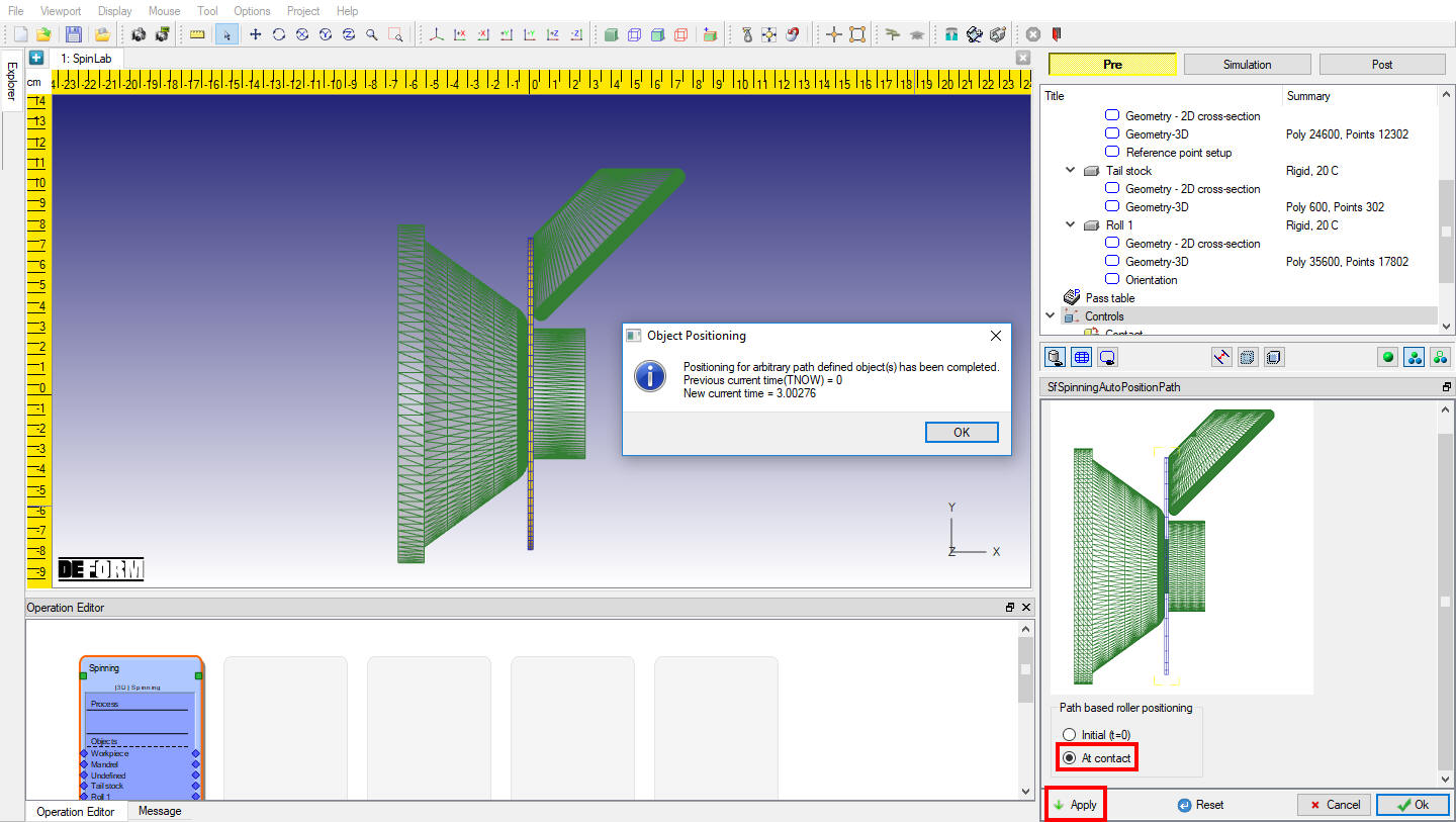
Automatic positioning window
Contact
In Contact page, select “User “ type and click on ![]() button. In table we will observe default relations being added, turn on sticking check box for Mandrel -Workpiece and Tail stock - Workpiece relations. Now define Shear friction value of 0.12 and click on
button. In table we will observe default relations being added, turn on sticking check box for Mandrel -Workpiece and Tail stock - Workpiece relations. Now define Shear friction value of 0.12 and click on ![]() button. Click on
button. Click on ![]() button to calculate default contact tolerance value and Generate contact by clicking on
button to calculate default contact tolerance value and Generate contact by clicking on ![]() button. Select Yes in “STICKING CONDITION” popup. Generated contact which looks like as shown in Fig. 3DSPL1.23. Click on
button. Select Yes in “STICKING CONDITION” popup. Generated contact which looks like as shown in Fig. 3DSPL1.23. Click on ![]() to Stopping controls page.
to Stopping controls page.
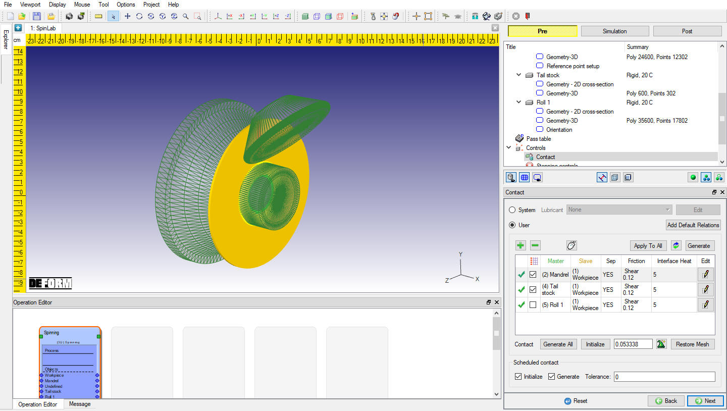
Contact page
Stopping Controls
Define Process Duration as 22 sec as shown in Fig. 3DSPL1.24. Click on ![]() to Simulation controls page.
to Simulation controls page.
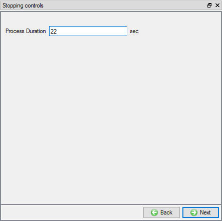
Process Duration page
Simulation controls
EnterNumber of steps as 999999 , Step increment to save as 50 and Time per step as 0.001 sec in Simulation controls page as shown in Fig. 3DSPL1.25. Click on ![]() to Generate DB page.
to Generate DB page.
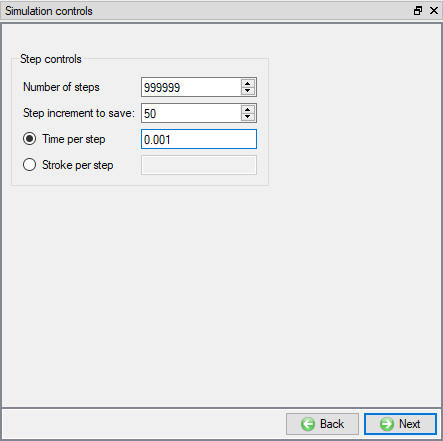
Simulation Controls page
Generate Database
In Generate DB page, click on the ![]() button to generate the database. Observe the message in Message tab informing database generation status.
button to generate the database. Observe the message in Message tab informing database generation status.
Running Simulation
Once the database has been generated, switch to the Simulation mode by selecting the ![]() button above the object tree. Click on the
button above the object tree. Click on the ![]() action label to open the Run Options dialog as shown in Fig. 3DSPL1.26.. Use the default Continue Run option to select “Continue from the last step ” option and then select the Simulation mode as Interactive and click on
action label to open the Run Options dialog as shown in Fig. 3DSPL1.26.. Use the default Continue Run option to select “Continue from the last step ” option and then select the Simulation mode as Interactive and click on ![]() button to run the simulation.
button to run the simulation.
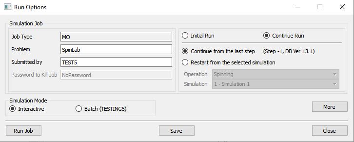
Run Simulation Window
Monitor the progress of the simulation by looking at the Simulation Message and Simulation Log tab, making sure that the ![]() option is checked. User can view the Spinning process as the simulation proceeds to the specified stopping criteria from Simulation graphics.
option is checked. User can view the Spinning process as the simulation proceeds to the specified stopping criteria from Simulation graphics.
Post processing
When the simulation is completed, review the results by switching to Post mode using the button above the Simulation tool bar.
Play through the steps of the simulation and look how the Workpiece part is formed during Spinning process.
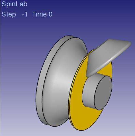
At step -1
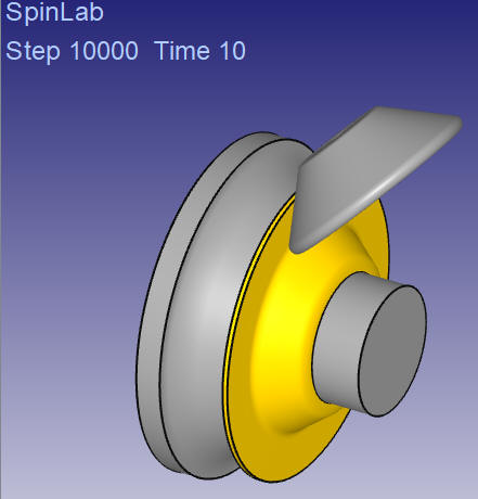
At Step 10000
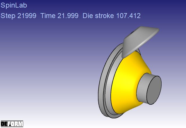
At last step
Plot Strain - Effective State variable and observe the Strain distribution.
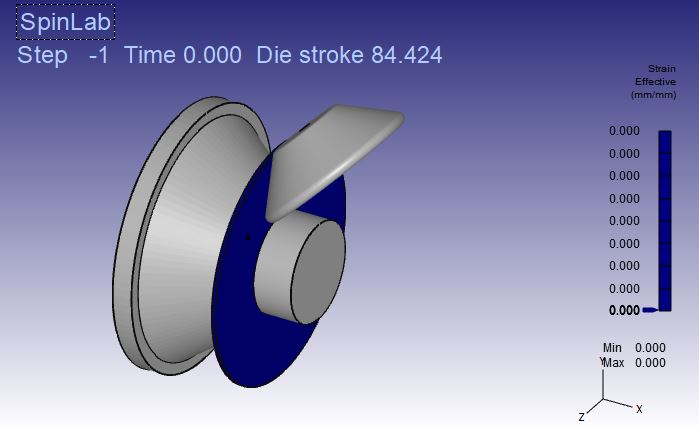
At step -1
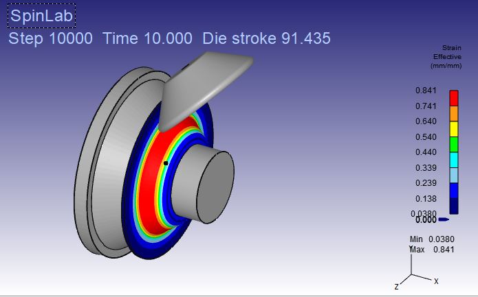
At step 10000
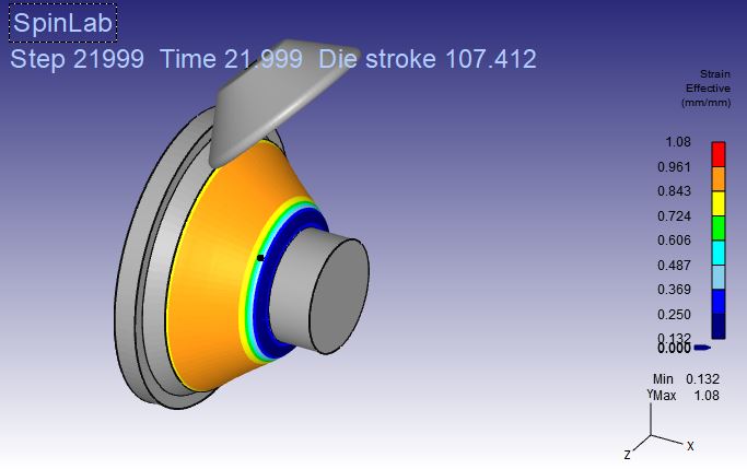
At last step