2D HT Lab 6 Grain Modeling
6.1. Introduction
6.2. Creating new project and Load Deformation Keyword File
6.3. Specify Grain-related Material Data
6.4. Input Initial Grain Variables
6.5. Generate DB and Run Deformation Simulation
6.6. Prepare and Run Air-cooling Simulation
6.7. Prepare and Run Water-Quenching Simulation
6.8. Post Processing
6.9. Changing Conditions
Introduction
The intent of the lab is to demonstrate how to use DEFORM Grain Model for simulating the grain microstructure evolution during forming and heat-treating processes.
Four evolution mechanisms are considered: static recrystallization, meta-dynamic recrystallization, dynamic recrystallization, and grain growth. Among these four mechanisms, dynamic recrystallization occurs during deformation, while the rest mechanisms occur during non-deforming periods. For each time step, based on current time, local temperature, strain, strain rate, and evolution history, the evolution mechanism is determined and the state variables are updated. Sixteen grain-related state variables are stored in the database, a detailed explanation of which is available in the User’s Manual. Recrystallization fraction and average grain sizes are usually of the most interest to users.
(Note: DEFORM grain model does not compute dynamic recrystallization simultaneously. Instead, the dynamic recrystallization that would have occurred during deformation is actually computed at the step immediately after the deformation. This means the users will not see any results unless the deformation simulation is followed by a non-deformation simulation, such as heat-treatment process. In addition, to simulate a complete microstructure evolution, the workpiece should be sufficiently cooled at the end of simulation.)
In this lab, a simple upsetting process is modeled, followed by air-cooling and water quenching. The problem is axisymmetric and uses SI units. The workpiece material is IN718, and the die material is steel H-13.
Creating new project and Load Deformation Keyword File
On a Windows machine , go to the ![]() button select DEFORM-v1x.xxx (.xxx indicates version number E.g. v14.0.2) and select DEFORM GUI Main vxx.xx from the menu. The DEFORM GUI Main window will appear, as shown below Fig. 2DHTML6.1.
button select DEFORM-v1x.xxx (.xxx indicates version number E.g. v14.0.2) and select DEFORM GUI Main vxx.xx from the menu. The DEFORM GUI Main window will appear, as shown below Fig. 2DHTML6.1.
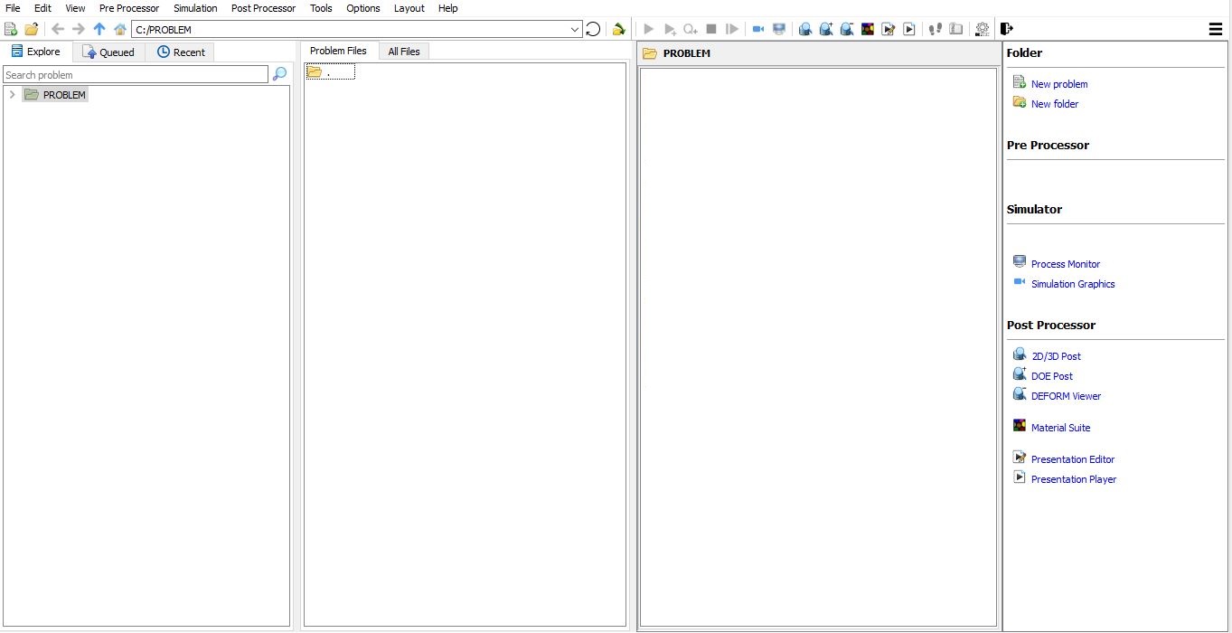
DEFORM GUI main window
Create a new problem either by selecting File![]() **New Problem** or by clicking the New Problem
**New Problem** or by clicking the New Problem ![]() icon. The Problem Setup window will appear as shown in Fig. 2DHTML6.2.Select “ Integrated Manufacturing Process “ radio button and units system as “SI “ using radio button. Define Problem Name as “GRAIN_LAB “ and make sure the “Show option dialog” check box is turned on (if we do not turn on the “Show option dialog ” check box, then we will not get the New Project dialog in MO UI). Then click on
icon. The Problem Setup window will appear as shown in Fig. 2DHTML6.2.Select “ Integrated Manufacturing Process “ radio button and units system as “SI “ using radio button. Define Problem Name as “GRAIN_LAB “ and make sure the “Show option dialog” check box is turned on (if we do not turn on the “Show option dialog ” check box, then we will not get the New Project dialog in MO UI). Then click on ![]() button to open a new Problem using the Deform Integrated Manufacturing Process.
button to open a new Problem using the Deform Integrated Manufacturing Process.
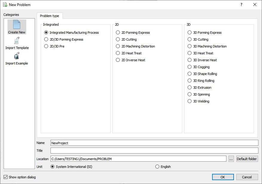
Problem type selection window
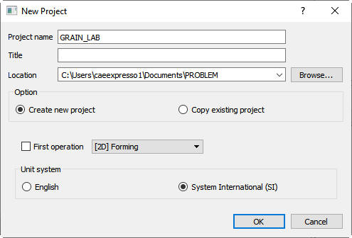
MO wizard will open along with project naming window, defined problem name is updated as ‘GRAIN_LAB ’ as the project name.(See Fig. 2DHTML6.3.).
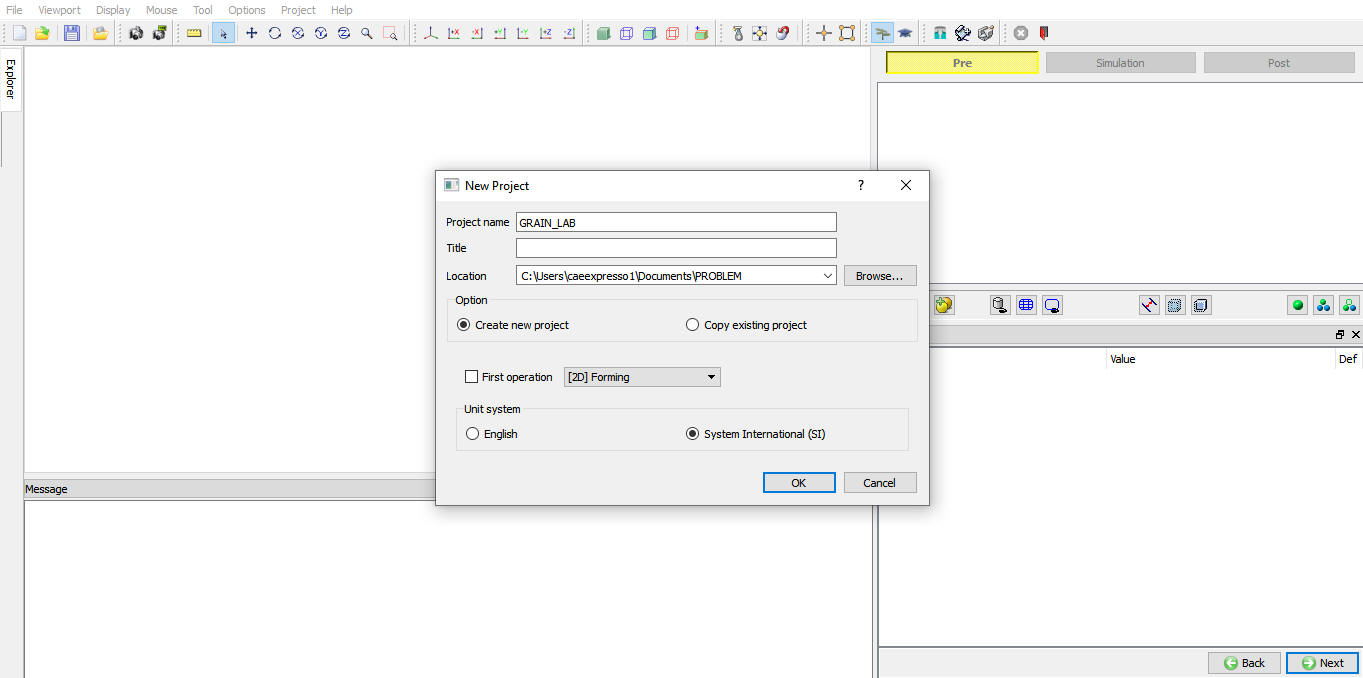
Problem location selection window
User can also change the Unit system (File menu selected unit system will be selected by default), for this lab we will select the SI unit system and we will add 2D Forming operation from Explorer operation list, so do not check “First operation” check box (see Fig. 2DHTML6.4.). Using copy Existing project option we can import previous saved projects as new project. Click on ![]() to continue to open the operation.
to continue to open the operation.
Assigning problem name
Multiple Operation wizard will open with new project called GRAIN_LAB. Add 2DForming operation from the Explorer Operations list. Add the operation by clicking on button next to 2D Forming or user can also add by drag and drop into the Operation Editor.(See Fig. 2DHTML6.5.)
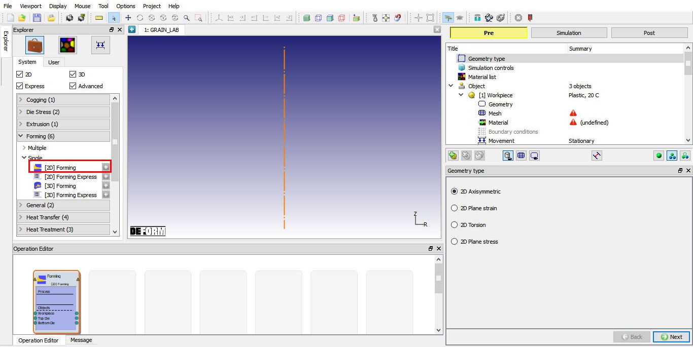
MO Wizard with 2D Forming Operation
Import keyword file GRN_UPSET.KEY from DEFORM/v*/2D/LABS directory. This keyword file contains all information for an upsetting forging simulation (see Fig. 2DHTML6.6.).
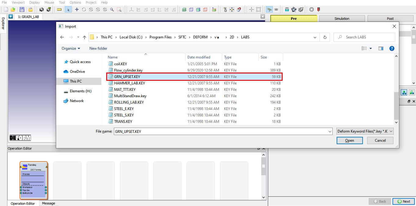
Importing key file
Specify Grain-related Material Data
Select the simulation control branch in operation tree, activate the Grain Check box. as shown in Fig. 2DHTML6.7.
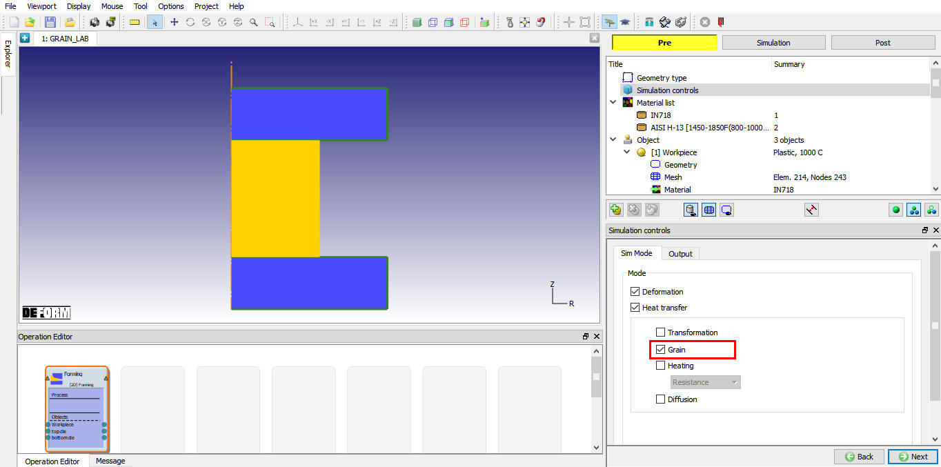
Activating Grain Check Box
Select the material IN718 branch under material list in operation tree. select the Avrami model in grain tab. Activate meta-dynamic Recrystallization and grain growth and deactivate the other two. Input the following data into the corresponding matrixes.
Peak Strain:
| Temp. | a1 | n1 | m1 | Q1 | c1 | a2 |
|---|---|---|---|---|---|---|
| 0 | 4.659e-3 | 0 | 0.1238 | 49520 | 0 | 0.83 |
Strain rate Boundary condition:
| Temp. | A | b1 | b2 | Q2 |
|---|---|---|---|---|
| 0 | 0.01 | 0 | 0 | 0 |
Meta-dynamic Recrystallization Kinetics:
| Temp. | a4 | H4 | n4 | m4 | Q4 | Beta_m | Km |
|---|---|---|---|---|---|---|---|
| 0 | 3.794e-9 | 0 | -1.42 | -0.408 | 196000 | 0.693 | 1 |
Meta-dynamic Recrystallization Grain Size:
| Temp. | a7 | h7 | n7 | m7 | Q7 | c7 |
|---|---|---|---|---|---|---|
| 0 | 4.85e10 | 0 | -0.41 | -0.028 | -240000 | 0 |
Grain Growth:
| Temp. | M | a9 | Q9 |
|---|---|---|---|
| 0 | 2 | 9.44e+19 | 467114.7 |
Input 300 for TemperatureLimit , under which the grain evolution is not computed. Keep 0 for StrainRetaining Co efficient.
Input Initial Grain Variables
Select the workpiece object, and click on Element Data ![]() icon. Click Grain tab under Microstructure. All grain variables can be defined and displayed here. Initialize both AverageGrainSize and InitialGrainSize with 100 as shown inFig. 2DHTML6.8., which is in unit µm. The Initial Grain Size stands for the unrecrystallized grain size. Note that you will need to use the Initialize button in order to input data for all elements at once. You may click Plot Variables
icon. Click Grain tab under Microstructure. All grain variables can be defined and displayed here. Initialize both AverageGrainSize and InitialGrainSize with 100 as shown inFig. 2DHTML6.8., which is in unit µm. The Initial Grain Size stands for the unrecrystallized grain size. Note that you will need to use the Initialize button in order to input data for all elements at once. You may click Plot Variables ![]() button to display and confirm the correct initializations.
button to display and confirm the correct initializations.
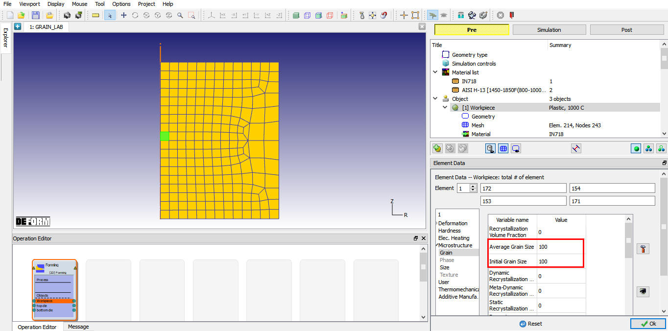
Defining Grain Variables
Generate DB and Run Deformation Simulation
In Generate DB page. Click the ![]() button to have the program check to see if anything was missed in the problem setup. During the checking process, messages in the red color signify data that needs to be fixed before a simulation can be run (such as when you forget to define any material data).
button to have the program check to see if anything was missed in the problem setup. During the checking process, messages in the red color signify data that needs to be fixed before a simulation can be run (such as when you forget to define any material data).
Click on ![]() button to generate the database. When the program is done writing the database, switch to
button to generate the database. When the program is done writing the database, switch to ![]() tab to run simulation.
tab to run simulation.
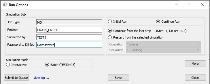
Click on the ![]() action label to open the Run Options dialog as shown in Fig. 2DHTML6.9. Use the default Continue Run option to select “Continue from the last step ” option and then select the Simulation mode as Interactive and click on
action label to open the Run Options dialog as shown in Fig. 2DHTML6.9. Use the default Continue Run option to select “Continue from the last step ” option and then select the Simulation mode as Interactive and click on ![]() button to run the simulation.
button to run the simulation.
Run Simulation window
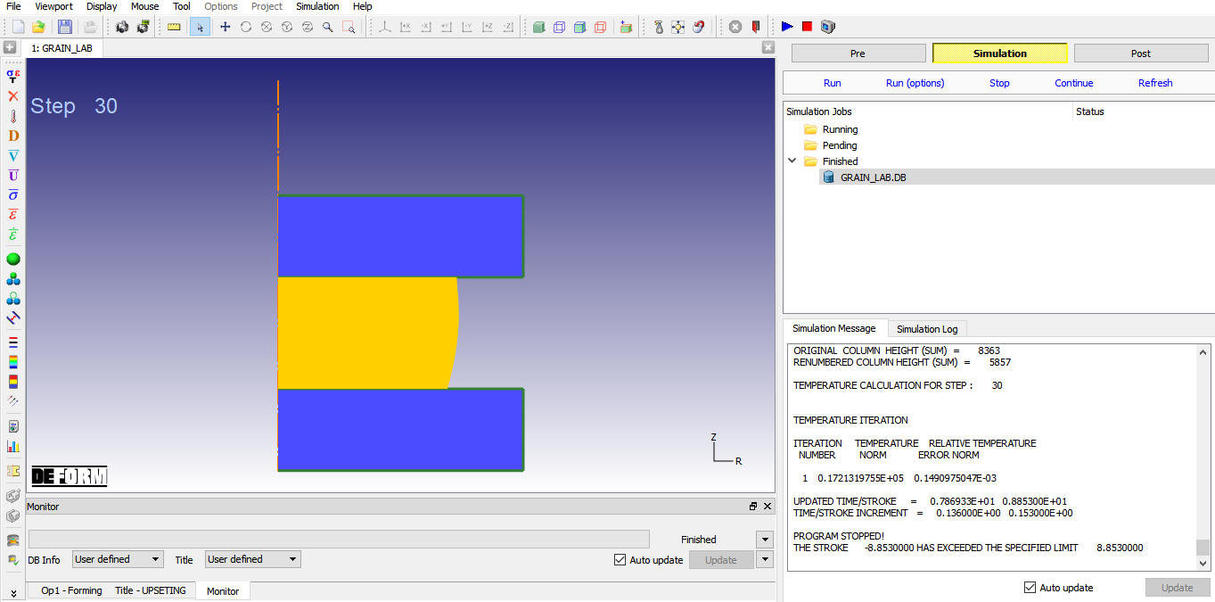
The progress of the simulation can be monitored as it is running by looking at the Simulation Message tab and Simulation Graphics from the Graphics display region in Simulation mode. As long as the ![]() option is checked in Simulation Message tab, which is the default setting, the Message file will refresh automatically.
option is checked in Simulation Message tab, which is the default setting, the Message file will refresh automatically.
The Message file provides information about which simulation step the simulation is currently on and also gives information dealing with how well the simulation is running.
When the simulation is finished without any issues, the following message will be added to the end of the Message file:”Program stopped!
The STROKE -8.8530000 HAS EXCEEDED THE SPECIFIED LIMIT 8.8530000”
Completion of the first operation
After completion of Simulation running, switch to ![]() button to add second operation.
button to add second operation.
Prepare and Run Air-cooling Simulation
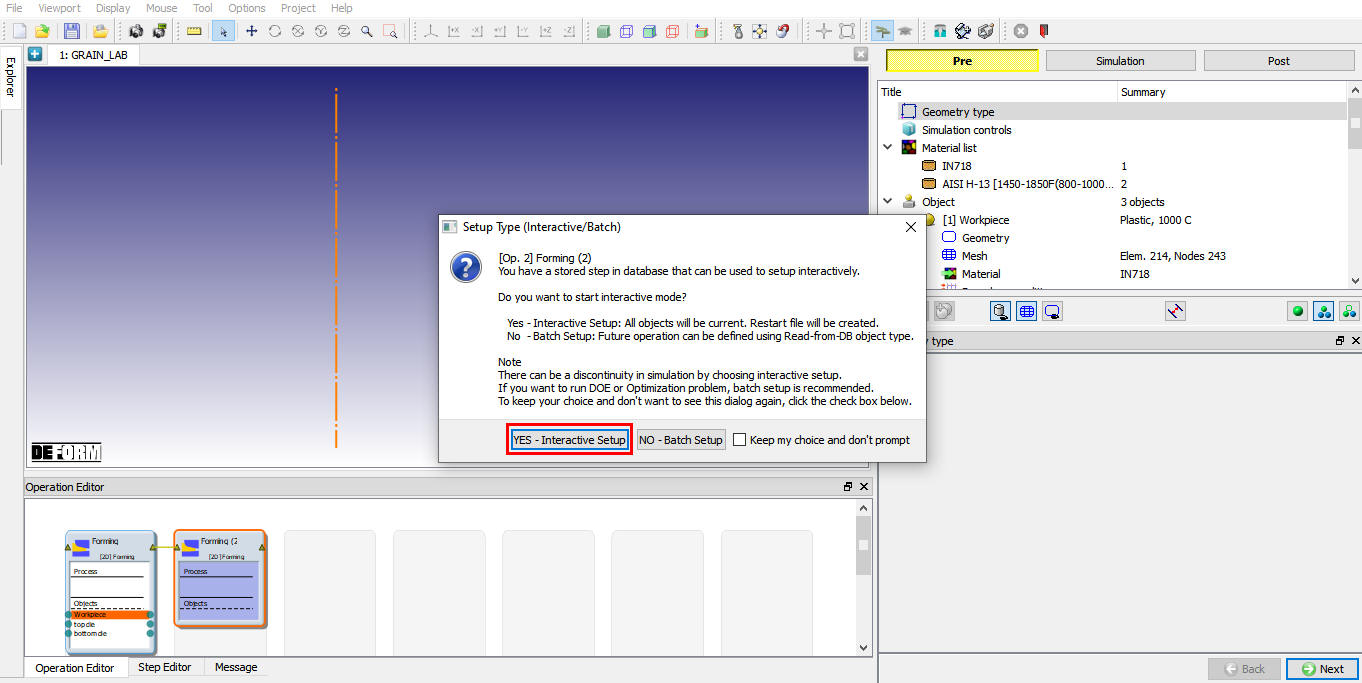
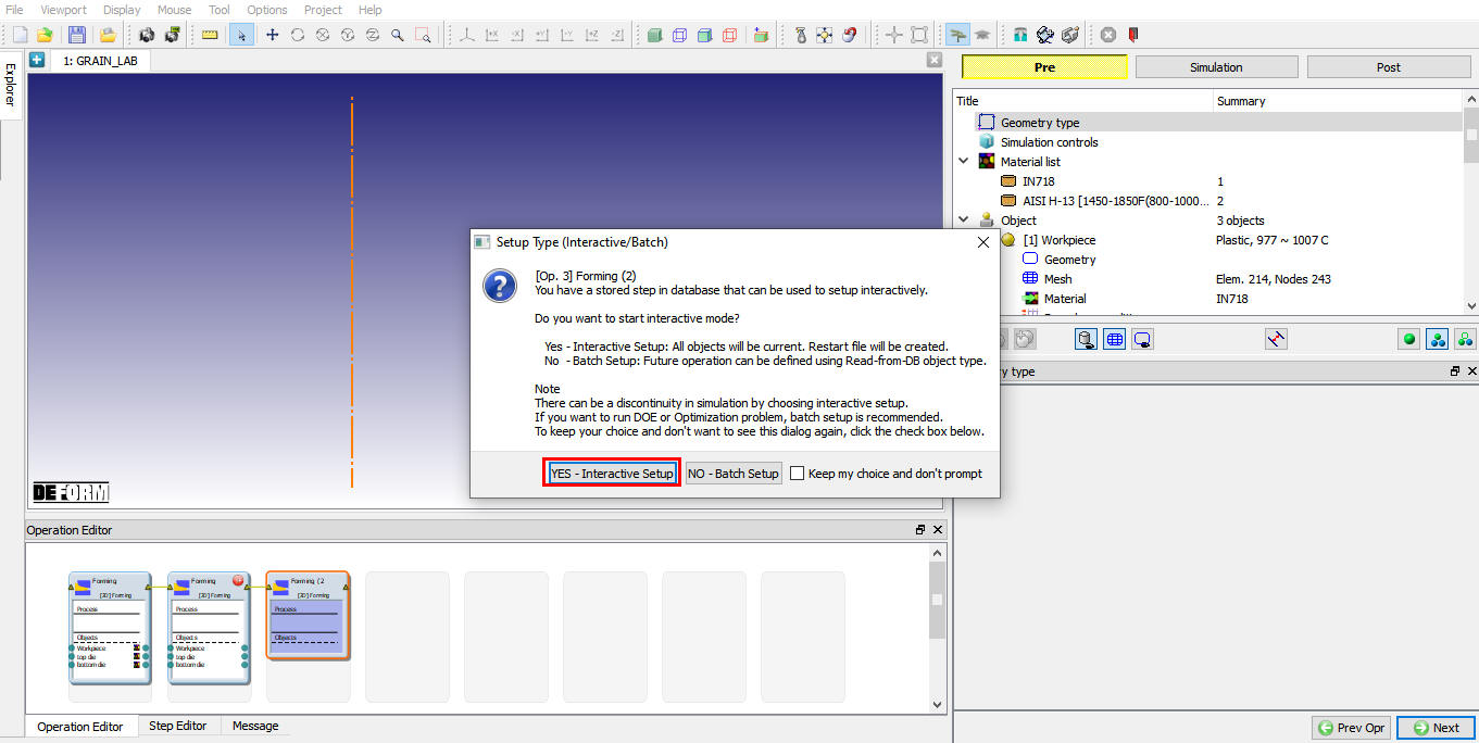
Add 2D forming operation from the Explorer Operation list. Then click on second forming operation to open second forming operation. When we click on second operation we will get Setup type popup, in popup click on ![]() button as shown in Fig. 2DHTML6.11.
button as shown in Fig. 2DHTML6.11.
Selecting Interactive setup type for second operation
Select the simulation control branch in operation tree, Turnoff the Deformation Check box as shown in Fig. 2DHTML6.12.
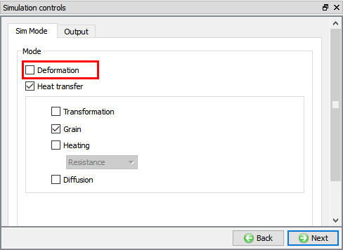
Simulation Control page
Select Top Die Movement branch and set the velocity to 0 as shown in Fig. 2DHTML6.13.
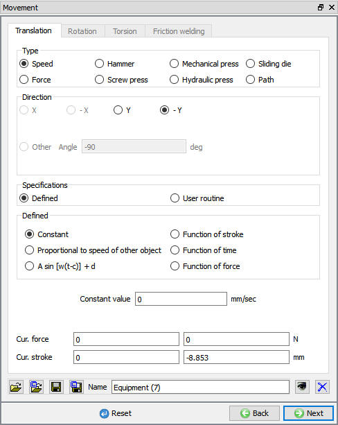
Deleting Top Die movement
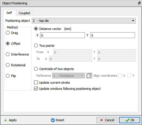
Click ![]() button under Controls branch. Offset the TopDie up by 5 mm as shown in Fig. 2DHTML6.14. Exit from Object Positioning dialog.
button under Controls branch. Offset the TopDie up by 5 mm as shown in Fig. 2DHTML6.14. Exit from Object Positioning dialog.
Object Positioning page
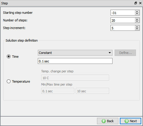
Select the Step control branch in operation tree, set solution Step Definition to ConstantTime Increment. Specify 0.1 seconds per step. number of simulationsteps to 20 and step increment to save to 5. This will model an air-cooling process of 2 seconds (See Fig. 2DHTML6.15.).
Simulation control page of second operation
Generate DB and Run the simulation for second operation as explained in the section 6.5
After the completion of simulation, switch to ![]() mode to add third forming operation.
mode to add third forming operation.
Prepare and Run Water-Quenching Simulation
Add 2D forming operation from the Explorer Operation list. Then click on third forming operation to open third forming operation. When we click on third operation we will get Setup type popup, in popup click on ![]() button as shown in Fig. 2DHTML6.16.
button as shown in Fig. 2DHTML6.16.
Selecting Interactive setup type for third operation
Click on ![]() button under Controls branch. Offset the BottomDie down by 5 mm as shown in Fig. 2DHTML6.17. Exit from Object Positioning dialog.
button under Controls branch. Offset the BottomDie down by 5 mm as shown in Fig. 2DHTML6.17. Exit from Object Positioning dialog.
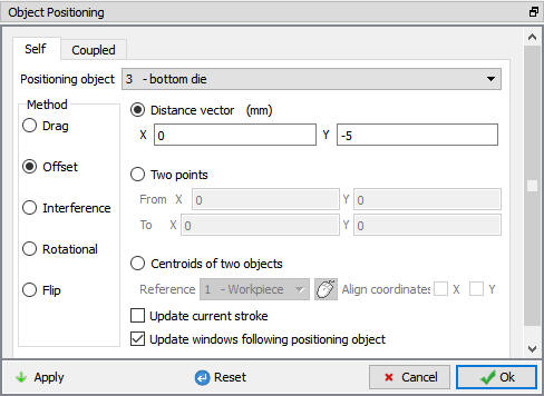
Positioning page for third operation
Select the Step control branch in operation tree, select ![]() icon to go to Expert mode. In ProcessingCondition tab, change the environmentalConvectioncoefficient to 15 for simulating water quenching.
icon to go to Expert mode. In ProcessingCondition tab, change the environmentalConvectioncoefficient to 15 for simulating water quenching.
In Step tab, set Numberofsimulationsteps to 100. set solution Step Definition to Constant Time Increment. Specify0.1 seconds per step (see Fig. 2DHTML6.18. and Fig. 2DHTML6.19.).
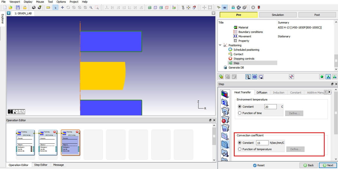
Defining Convection Coefficient
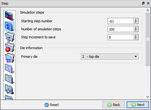
Simulation Control page for third operation
Generate DB and Run the simulation for second operation as explained in the section 6.5.
Post Processing
After simulation has been completed, switch to ![]() tab to view results, MO post processor will open.
tab to view results, MO post processor will open.
Open State Variable window and display Microstructure ![]() Grain Model
Grain Model ![]() Average Grain Size (see Fig. 2DHTML6.20.). (You may need to use Local scaling method in order to have a better display.) Note that, as mentioned previously, the effects of recrystallization will not show until deformation stage is over. Another important variable is the Rex. Vol. Fraction (see Fig. 2DHTML6.21.), which stands for the total volume fraction recrystallized. In this case, you can see that the bottom and up-right corner of the billet have relatively lower recrystallization, because of the lower strain. You can also display the recrystallized volume fraction and grain size from a particular mechanism, by clicking on corresponding state variables. Grain state variables are available also in Element Data. In addition, these results can be Point-Tracked.
Average Grain Size (see Fig. 2DHTML6.20.). (You may need to use Local scaling method in order to have a better display.) Note that, as mentioned previously, the effects of recrystallization will not show until deformation stage is over. Another important variable is the Rex. Vol. Fraction (see Fig. 2DHTML6.21.), which stands for the total volume fraction recrystallized. In this case, you can see that the bottom and up-right corner of the billet have relatively lower recrystallization, because of the lower strain. You can also display the recrystallized volume fraction and grain size from a particular mechanism, by clicking on corresponding state variables. Grain state variables are available also in Element Data. In addition, these results can be Point-Tracked.
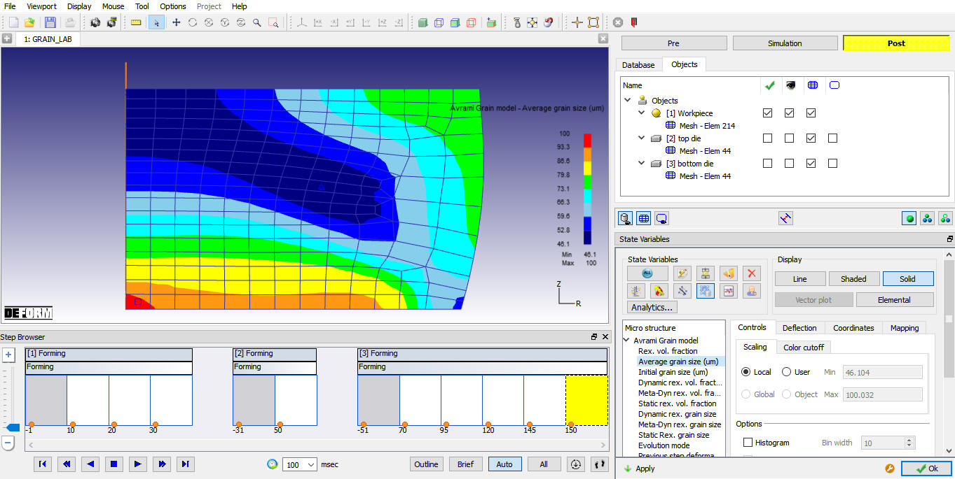
Avrami Grain Model - Average Grain size
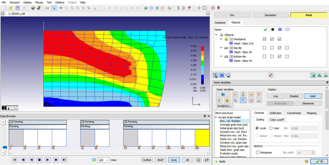
Avrami Grain Model - Rex. vol. fraction
Changing Conditions
It is often interesting to see how the final microstructure deviates if the processing conditions are changed. For example, you can modify the air-cooling duration from 2 seconds to 10 seconds and see a very different final grain size distribution. You can also increase the coefficient “a4” in the “Meta-dynamic Recrystallization Kinetics” to accelerate the recrystallization, etc. (If you are interested in additional grain-related material data, load “ WASPALOY1750- 2100F(950-1150C)” from the system material library).