Tube Flaring Lab
In this Lab we will setup simple Tube flaring operation in two stages.
-
Operation 1(Flair): In this lab we will perform Tube Flaring deformation operation using workpiece, punch and dies
-
Operation 2 (Unload): In this operation we will analyze the tube after unloading the tools upon completion of the Tube Flaring.
1.1. Operation 1: Flaring
1.1.1. Creating New problem
1.1.2. Adding 2D Forming Operation
1.1.3. Select Geometry type and Simulation Modes
1.1.4. Add material from Library
1.1.5. Adding Objects
1.1.6. Define Workpiece general object data
1.1.7. Create workpiece geometry from primitive
1.1.8. Generate Mesh for workpiece
1.1.9. Assign Material to Workpiece
1.1.10. Assign Workpiece boundary condition
1.1.11. Defining Top die object data
1.1.12. Import the Punch geometry
1.1.13. Assigning movement controls to Punch
1.1.14. Defining Bottom die object data
1.1.15. Import the Die geometry
1.1.16. Positioning objects
1.1.17. Define Inter-object relations
1.1.18. Define Stopping controls
1.1.19. Assign Step controls
1.1.20. Data checking and database generation
1.1.21. Run and monitor a simulation
1.2. Operation 2: Unload
1.2.1. Adding second Forming operation
1.2.2. Deleting Dies in Object page
1.2.3. Initializing Workpiece displacement value
1.2.4. Stopping controls page
1.2.5. Assign Step controls
1.2.6. Data checking and database generation
1.2.7. Run and monitor a simulation
1.2.8. Review Results
Operation 1: Flaring
Creating New problem
On a Windows machine, go to the ![]() button select DEFORM-v1x.xxx (.xxx indicates version number E.g. v14.0.2) and select DEFORM GUI Main v1x.x from the menu. The DEFORM GUI Main window will appear.
button select DEFORM-v1x.xxx (.xxx indicates version number E.g. v14.0.2) and select DEFORM GUI Main v1x.x from the menu. The DEFORM GUI Main window will appear.
Create a new problem either by selecting File![]() New Problem or by clicking the New Problem
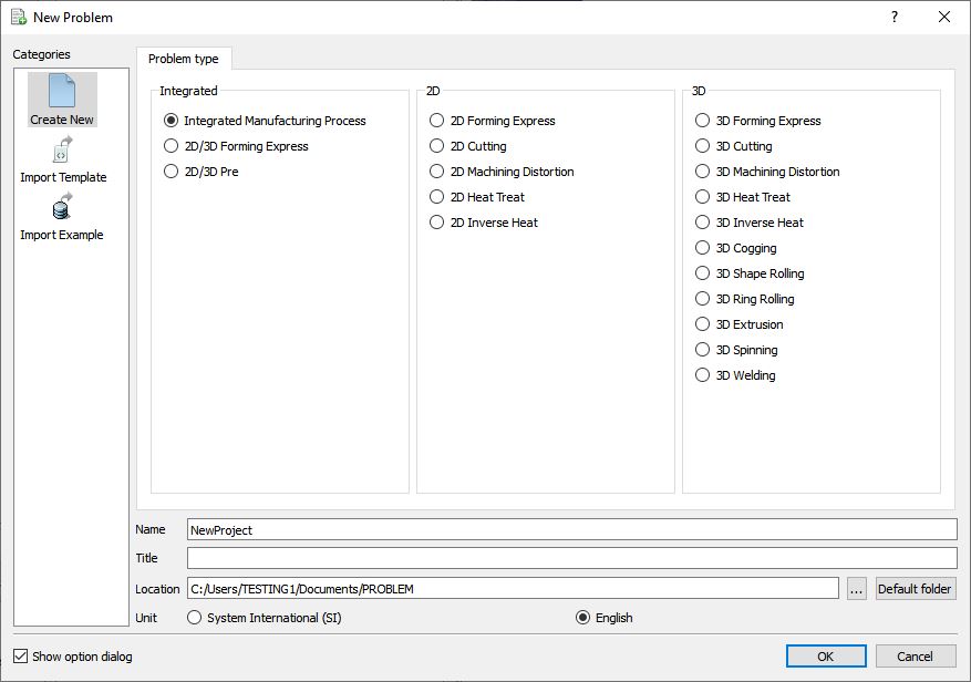
New Problem or by clicking the New Problem ![]() icon. The Problem Setup window will appear as shown in Fig. 2DTFL1.1. Select “ Integrated Manufacturing Process “ radio button and unit system as “English “ radio button in unit field. Define Problem Name as “ **Tube_Flaring** “ and make sure the “Show option dialog ” check box is turned on (if we do not turn on the “Show option dialog” check box, then we will not get the New Project dialog). Then click on
icon. The Problem Setup window will appear as shown in Fig. 2DTFL1.1. Select “ Integrated Manufacturing Process “ radio button and unit system as “English “ radio button in unit field. Define Problem Name as “ **Tube_Flaring** “ and make sure the “Show option dialog ” check box is turned on (if we do not turn on the “Show option dialog” check box, then we will not get the New Project dialog). Then click on ![]() button to open a new problem using the Deform Integrated Manufacturing Process.
button to open a new problem using the Deform Integrated Manufacturing Process.
Problem Setup Window
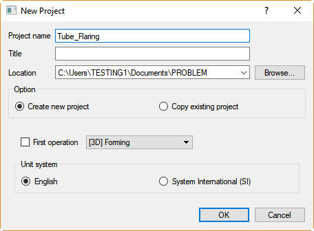
Multiple operation wizard will opens along with New Project window, retain the project name as Tube_Flaring and confirm that First operation check box is unchecked as we will add operation later and use the default (home) directory as problem location as shown in Fig. 2DTFL1.2. Click ![]() to open new project.
to open new project.
New MO Project window
Adding 2D Forming Operation
Multiple Operation wizard will open a new project. Add 2D Forming operation from the Explorer Operations list. Operation can be added by clicking on 2D Forming operation ![]() button (See Fig. 2DTFL1.3.) or user can also add by drag and drop into the Operation Editor.
button (See Fig. 2DTFL1.3.) or user can also add by drag and drop into the Operation Editor.
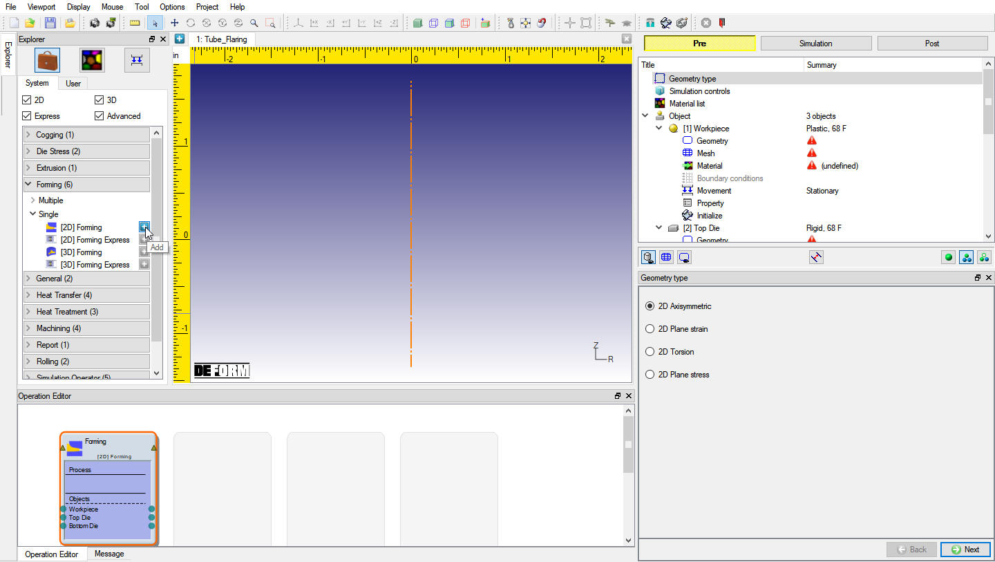
Adding 2D Forming operation from operation explorer
Change the default operation title to “Flaring “ from Forming by selecting the title in the operation editor as shown in Fig. 2DTFL1.4 and press Enter keyboard button.
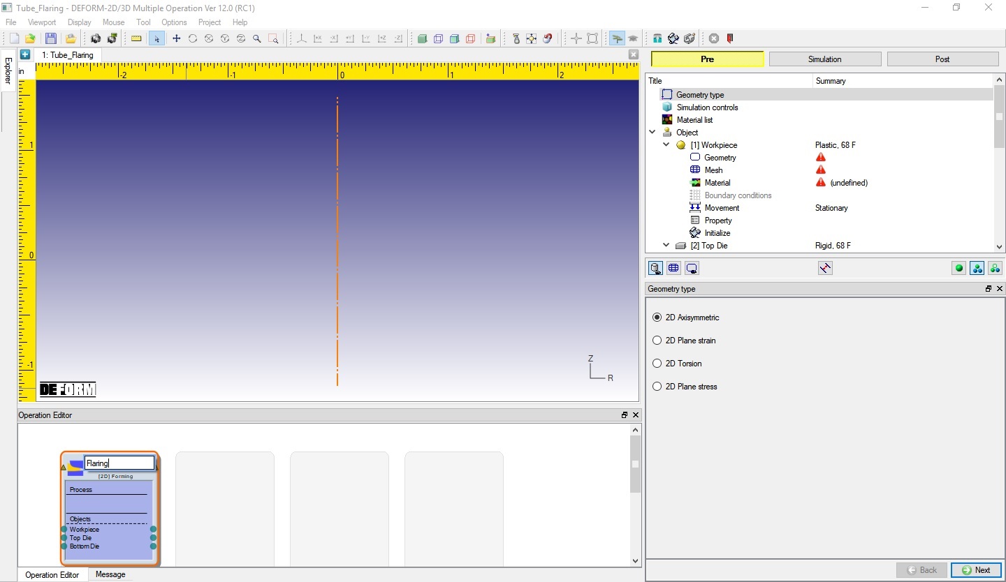
Renaming operation title to Flaring
Select Geometry type and Simulation Modes
Confirm the geometry type selected is Axi-symmetric in Geometry type page, then click![]() .
.
In this lab we will be showing how to setup simple Isothermal problem, so in Simulation controls page, uncheck the Heat transfer mode check box (See Fig. 2DTFL1.5), then click ![]() .
.
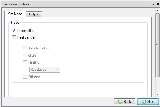
Simulation control window
Add material from Library
Click the ![]() (Load material from library) button as shown in Fig. 2DTFL1.6. Select the Steel category, then select AISI-1010,COLD[70F(20C)] and click the
(Load material from library) button as shown in Fig. 2DTFL1.6. Select the Steel category, then select AISI-1010,COLD[70F(20C)] and click the ![]() button.
button.
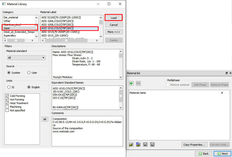
Loading material from library
Material is loaded to material list, click ![]() .
.
To improve convergence in cold material we will edit material properties. Click the ![]() next to Flow Stress. Select the strainrate “100 ” field and delete it (See Fig. 2DTFL1.7.). This leaves a single strain rate which is reasonable and better for convergence. Click
next to Flow Stress. Select the strainrate “100 ” field and delete it (See Fig. 2DTFL1.7.). This leaves a single strain rate which is reasonable and better for convergence. Click ![]() .
.
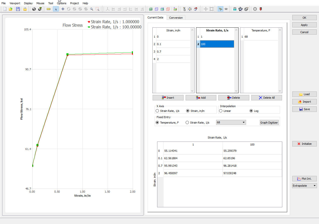
Editing Material Flow stress data
Adding Objects
The Flaring operation to be simulated requires a workpiece, top and bottom die. By default, three objects will be added in Forming operation list, if not added click the ![]() (insert object) button three times to add 3 objects to list, Workpiece and two dies. Object window looks as shown in Fig. 2DTFL1.8. Click
(insert object) button three times to add 3 objects to list, Workpiece and two dies. Object window looks as shown in Fig. 2DTFL1.8. Click ![]() button.
button.
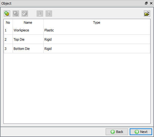
Objects window to Add or Delete the objects
Define Workpiece general object data
Accept the default object name Workpiece. Assign the temperature as 70 °F and select the object type as Elasto-plastic. (See Fig. 2DTFL1.9.). Click ![]() button.
button.
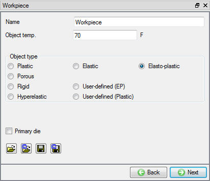
Workpiece object window
Create workpiece geometry from primitive
Click on the ![]() button to create a geometry within DEFORM. The workpiece Outer diameter is 2.2”, Inner diameter is 2” and Height is 3”, so you will define a width of half the diameter. Select Hollowcylinder , enter Innerradius as 1, Outerradius as 1.1. and Height as 3 , (See Fig. 2DTFL1.10.). Click on
button to create a geometry within DEFORM. The workpiece Outer diameter is 2.2”, Inner diameter is 2” and Height is 3”, so you will define a width of half the diameter. Select Hollowcylinder , enter Innerradius as 1, Outerradius as 1.1. and Height as 3 , (See Fig. 2DTFL1.10.). Click on ![]() button and then observe the geometry in graphics window. Click
button and then observe the geometry in graphics window. Click ![]() button to generate workpiece mesh.
button to generate workpiece mesh.
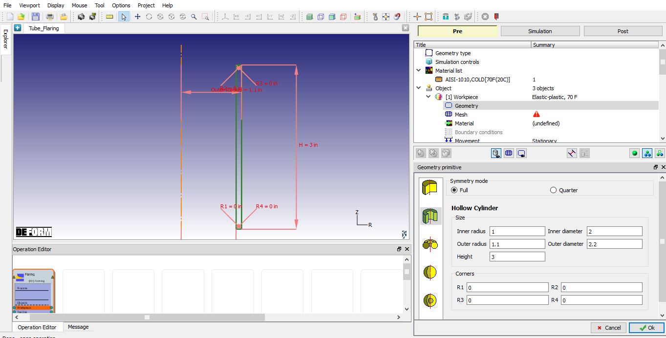
2D axi-symmetric geometry primitive window
Generate Mesh for workpiece
We will generate Mapped mesh with 350 elements and** 4** elements in Thickness direction. So, click on ![]() icon to switch to expert mode. Define Targetnumberofelements as 350 , Thickness elements as 4 , check Mapped mesh check box and click the
icon to switch to expert mode. Define Targetnumberofelements as 350 , Thickness elements as 4 , check Mapped mesh check box and click the ![]() button to generate the mesh for workpiece as shown in Fig. 2DTFL1.11. Click
button to generate the mesh for workpiece as shown in Fig. 2DTFL1.11. Click ![]() button to assign material for workpiece.
button to assign material for workpiece.
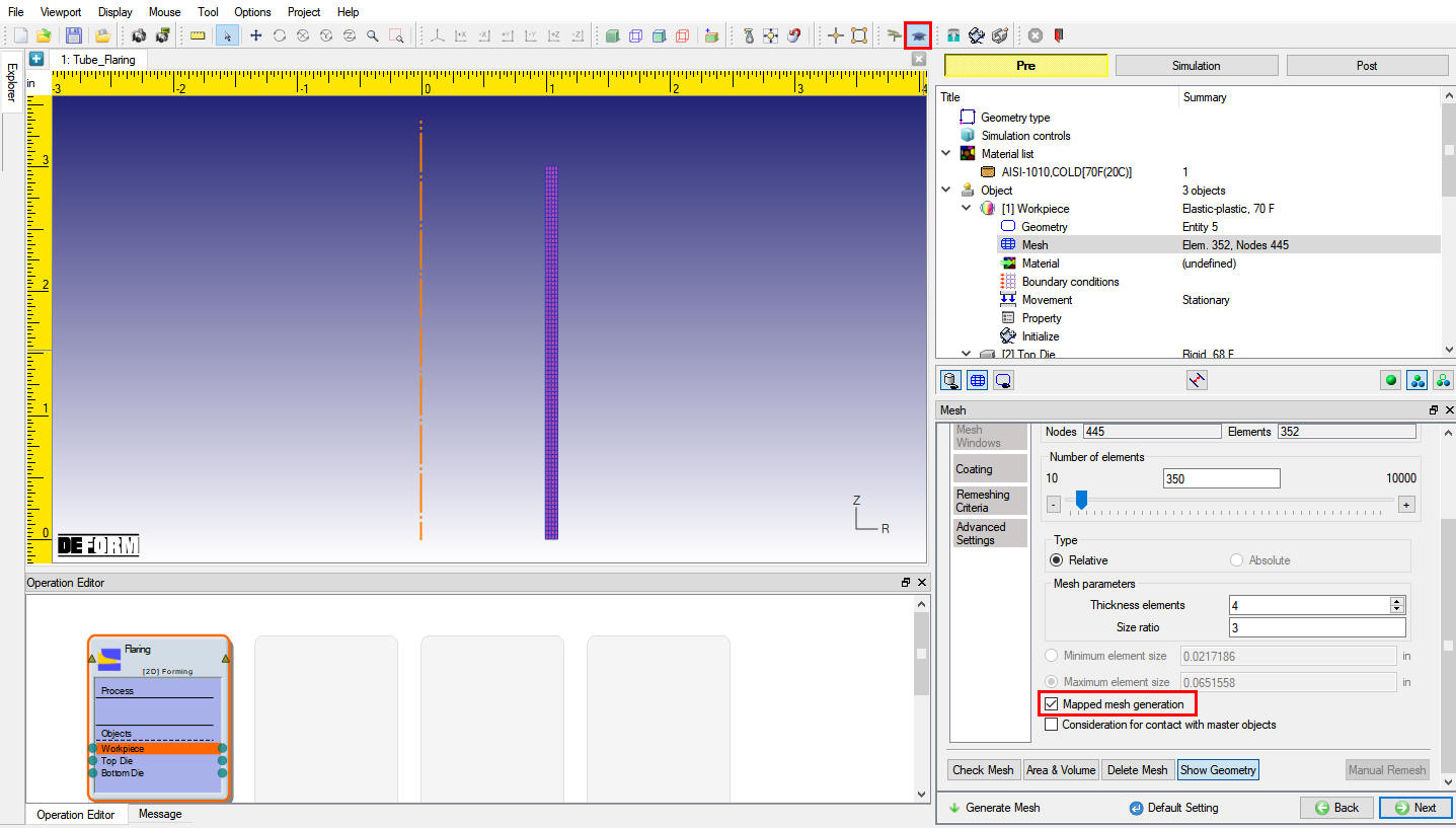
Expert mode mesh window
Assign Material to Workpiece
Select theAISI-1010,COLD[70F(20C)] in the material window to assign the material to the workpiece. Click ![]() button to assign the workpiece boundary conditions.
button to assign the workpiece boundary conditions.
Assign Workpiece boundary condition
Assign Vy=0 boundary conditions to the bottom edge of the workpiece as shown in Fig. 2DTFL1.12. Click ![]() button until Top die page.
button until Top die page.
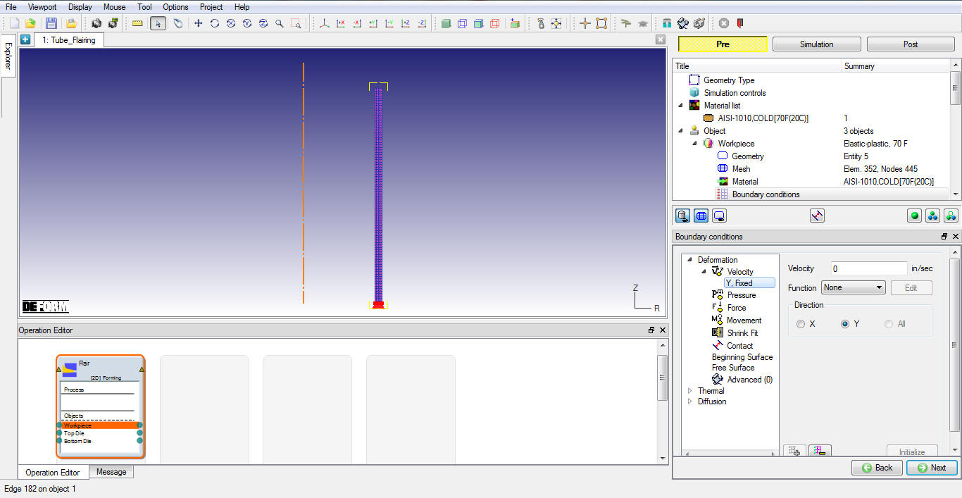
Assigning BCC for Workpiece
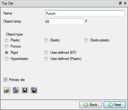
Defining Top die object data
Change the Object name to “Punch “, Keep the Top die default temperature as 68 ° F and confirm the object type selected is rigid and Primary die check box is turned on as shown in Fig. 2DTFL1.13. Click ![]() to Punch geometry page.
to Punch geometry page.
Top die window
Import the Punch geometry
Click the ![]() (Load geometry from a file) button and import the file “FlarePunch.IGS” by browsing the geometry file path located in DEFORM installation folder \Tutorials directory. Check the geometry using
(Load geometry from a file) button and import the file “FlarePunch.IGS” by browsing the geometry file path located in DEFORM installation folder \Tutorials directory. Check the geometry using ![]() option to make sure the geometry is OK. Click
option to make sure the geometry is OK. Click ![]() until Punch movement page.
until Punch movement page.
Assigning movement controls to Punch
The default mode is constant speed. Input a value of 5 in/sec for the Constant value and confirm that the Direction is -Y as shown in Fig. 2DTFL1.14. Click ![]() until Bottom die page.
until Bottom die page.
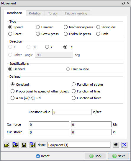
Punch movement window
Defining Bottom die object data
Change the Object name to “Die “, Keep the Top die default temperature as 68 ° F and confirm the object type selected is rigid. Click ![]() to Die geometry page.
to Die geometry page.
Import the Die geometry
Click the ![]() (Load geometry from a file) button and import the file “FlareDie.IGS ” by browsing the geometry file path located in DEFORM installation folder \Tutorials directory. Check the geometry using
(Load geometry from a file) button and import the file “FlareDie.IGS ” by browsing the geometry file path located in DEFORM installation folder \Tutorials directory. Check the geometry using ![]() option to make sure the geometry is OK. Click
option to make sure the geometry is OK. Click ![]() until Positioning page.
until Positioning page.
Positioning objects
The geometries should be in the correct position. Confirm that the workpiece is positioned on top of the bottom die and that the top die is positioned against the workpiece. Further positioning is not required for this operation. Click ![]() until Contact page.
until Contact page.
Define Inter-object relations
Assign the default inter-object relationships using ![]() button. The workpiece should be slave to both the Punch and Die. Click on the
button. The workpiece should be slave to both the Punch and Die. Click on the ![]() button for one of the relationships. Select Coulombtype friction radio button, define 0.1 value. Click
button for one of the relationships. Select Coulombtype friction radio button, define 0.1 value. Click ![]() to exit the menu. Click
to exit the menu. Click ![]() to apply the friction value to the two other relationships. (See Fig. 2DTFL1.15.). Click
to apply the friction value to the two other relationships. (See Fig. 2DTFL1.15.). Click ![]() to Stopping controls page.
to Stopping controls page.
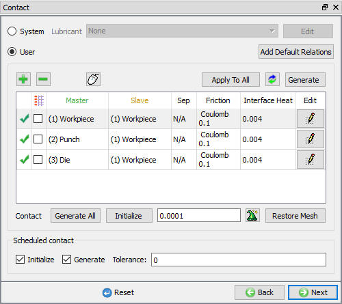
Inter - object Relation window
Define Stopping controls
Click on ![]() mode icon to switch to Guided mode. Assign Max die stroke value as 1.14 “ in Y direction by checking Max die stroke check box as shown in Fig. 2DTFL1.16. Click
mode icon to switch to Guided mode. Assign Max die stroke value as 1.14 “ in Y direction by checking Max die stroke check box as shown in Fig. 2DTFL1.16. Click ![]() to Step page.
to Step page.
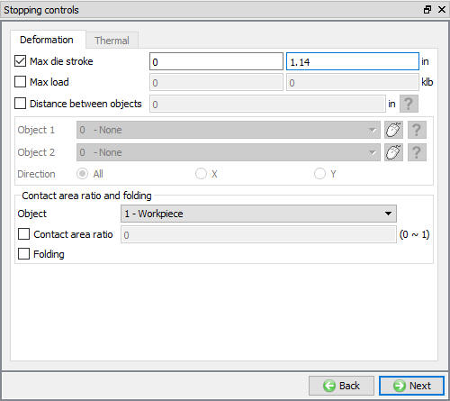
Stopping controls window
Assign Step controls
The tool needs to move by 1.2’’ to produce the desired shape and die displacement per step = 10% of element edge length. The element edge length is 0.025” when measured, So the Number of Simulation Steps is equal to 1.2”/(10% of 0.025”). Hence define Number of Steps as 480 , Step increment as 5 and die displacement per step as 0.0025 , see Fig. 2DTFL1.17. Click ![]() to Generate DB page.
to Generate DB page.
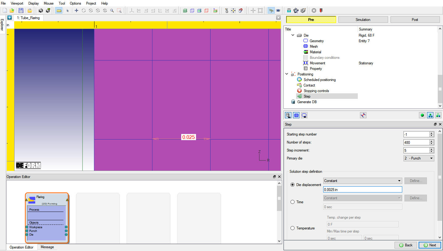
Step controls window
Data checking and database generation
Click on the ![]() button, the data checking system will confirm that defined data is appropriate for running a simulation.
button, the data checking system will confirm that defined data is appropriate for running a simulation.
Red marks indicate missing or incorrect data that will prevent a simulation from running. It is necessary to correct those errors before the database can be generated.
Yellow marks indicate data which may be suspect and should be reviewed. These should be investigated carefully, as they might result in system instability or erroneous (incorrect) results.
Review the data checking information. If there are no yellow or red marks, click the ![]() button.
button.
You should look for the words: Database has been generated. When you see this, it means that your inputs have been saved to the database and you are now ready to run the simulation.
Click on the MO ![]() Mode button (above the operation tree) to start the simulation.
Mode button (above the operation tree) to start the simulation.
Run and monitor a simulation
Click on the ![]() action label to open the Run Options dialog. Use the default Continue Run option to select “Continue from the last step ” option and then select the Simulation mode as Interactive and click on
action label to open the Run Options dialog. Use the default Continue Run option to select “Continue from the last step ” option and then select the Simulation mode as Interactive and click on ![]() button to run the simulation.
button to run the simulation.
The progress of the simulation can be monitored as it is running by looking at the Simulation Message tab and Simulation Graphics from the Graphics display region in Simulation mode. If ![]() option is checked in Simulation Message tab, which is the default setting, the Message file will refresh automatically.
option is checked in Simulation Message tab, which is the default setting, the Message file will refresh automatically.
The Message file provides information about which simulation step the simulation is currently on and information dealing with how well the simulation is running as shown in Fig. 2DFRCL2.18.
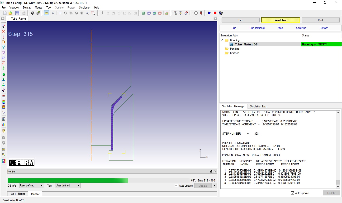
Running the simulation from MO simulation mode
After completion of simulation, click on ![]() MO mode button to switch to Pre mode and continue to setup the next operation.
MO mode button to switch to Pre mode and continue to setup the next operation.
Operation 2: Unload
Adding second Forming operation
In this operation we will perform Springback analysis by unloading in 2D Forming operation.
Add 2D Forming operation from the Explorer Operations list. Operation can be added by clicking on 2D Forming operation ![]() button or user can also add by drag and drop into the Operation Editor.
button or user can also add by drag and drop into the Operation Editor.
Select the 2D Forming operation from operation editor to open the 2D forming operation. Select the ![]() button for Setup type popup (See Fig. 2DTFL1.19.) to setup the problem in batch mode.
button for Setup type popup (See Fig. 2DTFL1.19.) to setup the problem in batch mode.
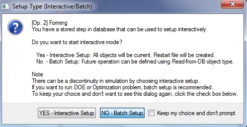
Selecting Batch mode type setup
Change the default operation title to “Unload “ from Forming by selecting the title in the operation editor as shown in Fig. 2DTFL1.20. and press Enter keyboard button after editing the table. Click ![]() until Object page.
until Object page.
Renaming operation title to Unload
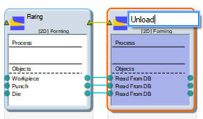
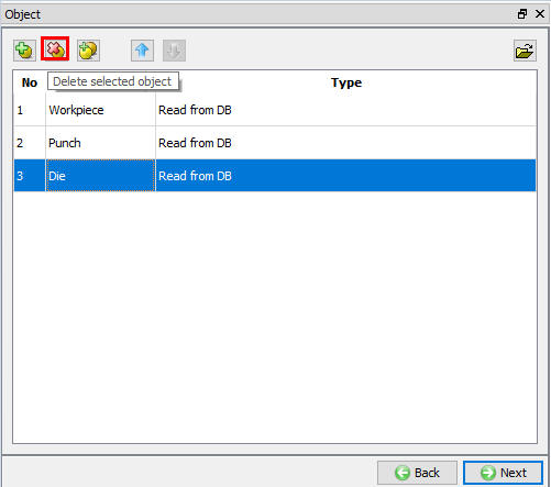
Deleting Dies in Object page
Delete Punch and Die from the list using ![]() button (See Fig. 2DTFL1.21.). Click
button (See Fig. 2DTFL1.21.). Click ![]() until workpiece Initialize page.
until workpiece Initialize page.
Deleting Punch and Die using Delete button in Object window
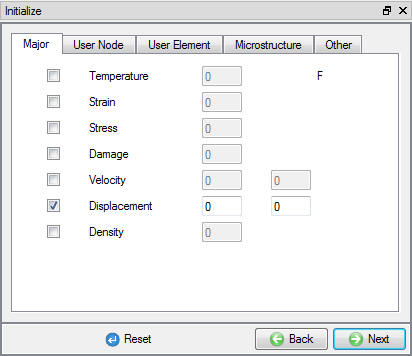
Initializing Workpiece displacement value
Turn on the Displacement Checkbox and use default 0 value to initialize (See Fig. 2DTFL1.22.). Click ![]() until Stopping controls page.
until Stopping controls page.
Workpiece Initialize window
Stopping controls page
Ensure that the stroke stopping criteria is initialized i.e., turned off. Click ![]() to Step page.
to Step page.
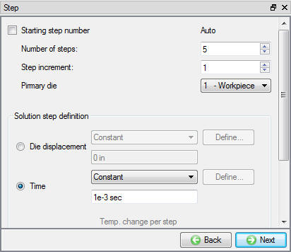
Assign Step controls
Assign the Number of steps as 5 , Step increment as 1 and time increment as 1e-3 seconds (See Fig. 2DTFL1.23.)).
Step controls window
Data checking and database generation
Click on the ![]() button, the data checking system will confirm that defined data is appropriate for running a simulation.
button, the data checking system will confirm that defined data is appropriate for running a simulation.
Red marks indicate missing or incorrect data that will prevent a simulation from running. It is necessary to correct those errors before the database can be generated.
Yellow marks indicate data which may be suspect and should be reviewed. These should be investigated carefully, as they might result in system instability or erroneous (incorrect) results.
Review the data checking information. If there are no yellow or red marks, click the ![]() button.
button.
You should look for the words: Database has been generated. When you see this, it means that your inputs have been saved to the database and you are now ready to run the simulation.
Click on the MO ![]() Mode button (above the operation tree) to start the simulation.
Mode button (above the operation tree) to start the simulation.
Run and monitor a simulation
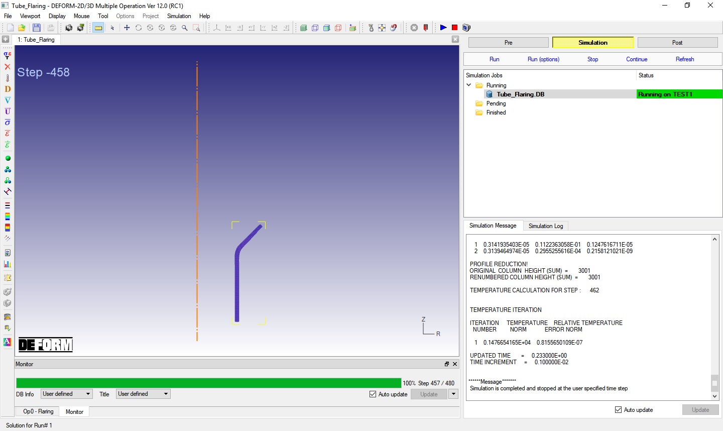
Once the database has been generated, switch to the Simulation mode by clicking on ![]() button above the operation tree. Click on the
button above the operation tree. Click on the ![]() action label to open the Run Options dialog. Use the default Continue Run option to select “Continue from the last step ” option and then select the Simulation mode as Interactive and click on
action label to open the Run Options dialog. Use the default Continue Run option to select “Continue from the last step ” option and then select the Simulation mode as Interactive and click on ![]() button to run the simulation.
button to run the simulation.
Watching the simulation graphics provides an initial idea of what to expect when opening the postprocessor. Also monitor simulation from Simulation and log messages. The message file and log file will indicate that the simulation has been completed on the last line, confirming that click on ![]() Mode button to review results.
Mode button to review results.
Monitoring the simulation in Simulation mode
Review Results
State variables:
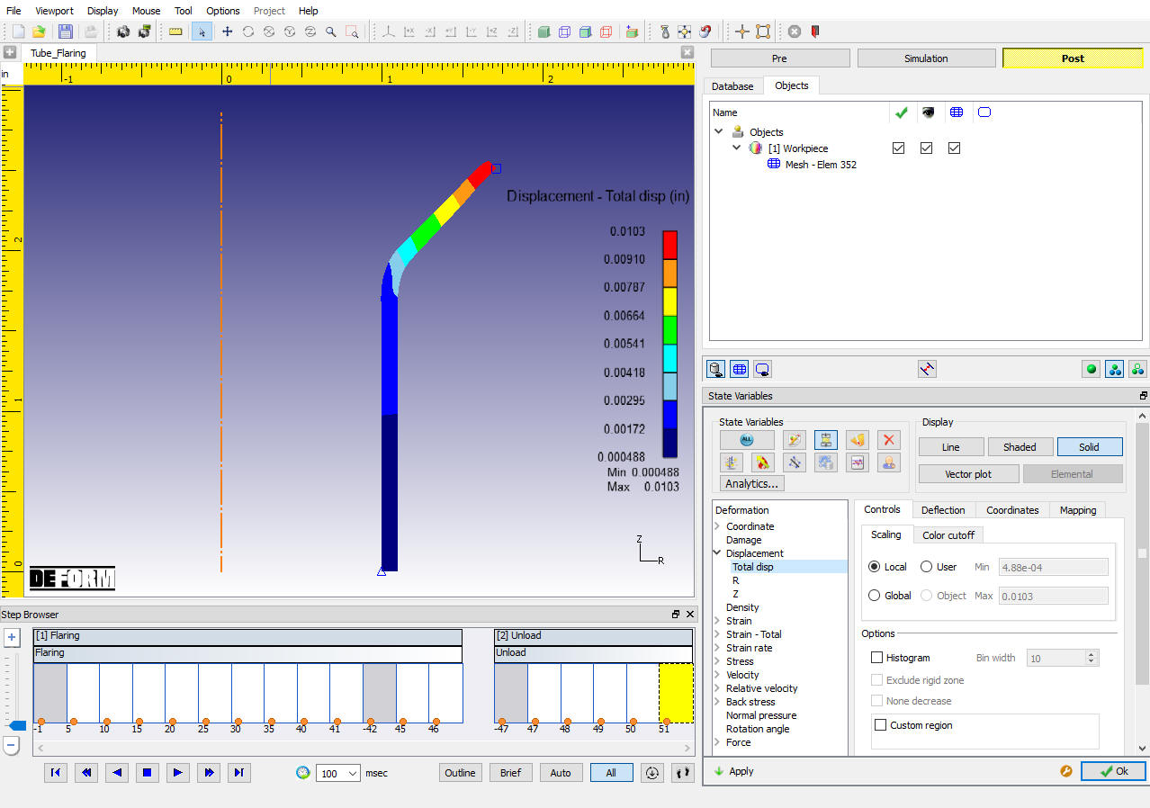
To view the spring back, open state variable dialog ![]() and plot total displacement from displacement. Click on Deflection tab and select the Use Deflection checkbox on the “State Variables” dialog. The workpiece with magnified distortion is shown in Fig. 2DTFL1.25. Use the slide bar to increase or decrease the exaggeration of distortion.
and plot total displacement from displacement. Click on Deflection tab and select the Use Deflection checkbox on the “State Variables” dialog. The workpiece with magnified distortion is shown in Fig. 2DTFL1.25. Use the slide bar to increase or decrease the exaggeration of distortion.
Total-Displacement state variable with Deflection
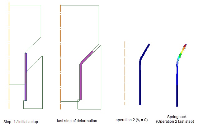
Tube Flaring operation Workpiece shape in each operation first and last step