Lab 5. Stub Shaft Labs
5.1. Operation1: Cone Operation
5.2. Operation2: Head Operation
5.3. Symmetry/Thermal Operations
5.4. Tool Stress Analysis
5.5. Adding a Shrink ring to the die
5.6. Mechanical Press
Operation1: Cone Operation
Creating New Problem
Create a new problem either by selecting File![]() **New Problem** or by clicking the NewProblem
**New Problem** or by clicking the NewProblem![]() icon. The Problem Setup window will appear. Select “Integrated Manufacturing Process “ radio button and units system as “English “ radio button in units field. Define Problem Name as “Stub_Shaft “ and make sure the “Show option dialog ” check box is turned on (if we do not turn on the “Show option dialog” check box, then we will not get the New Project dialog). Then click on
icon. The Problem Setup window will appear. Select “Integrated Manufacturing Process “ radio button and units system as “English “ radio button in units field. Define Problem Name as “Stub_Shaft “ and make sure the “Show option dialog ” check box is turned on (if we do not turn on the “Show option dialog” check box, then we will not get the New Project dialog). Then click on ![]() button to open a new problem using the Deform Integrated Manufacturing Process.
button to open a new problem using the Deform Integrated Manufacturing Process.
MO wizard will open, at this point user will be prompted to specify a project name (system will create a separate folder with this project name) and title for this session. In this session we use ‘Stub_Shaft ’ as the project name.
User can also change the Unit system and add operation by selecting from First operation pull down list and checkbox. Using copy Existing project option we can import previous saved projects as new project. Click on ![]() to continue to open the operation.
to continue to open the operation.
Adding operations
Add two3DFormingoperations from the Explorer Operations list. Add the operations by clicking on 3D Forming ![]() button or user can also add by drag and drop into the Operation Editor.
button or user can also add by drag and drop into the Operation Editor.
Simulation Controls
In this lab we will be showing how to setup simple Isothermal problem. So in Simulation controls uncheck the Heattransfer mode check box (see Fig. 3DL5.1.). Then click on ![]() .
.
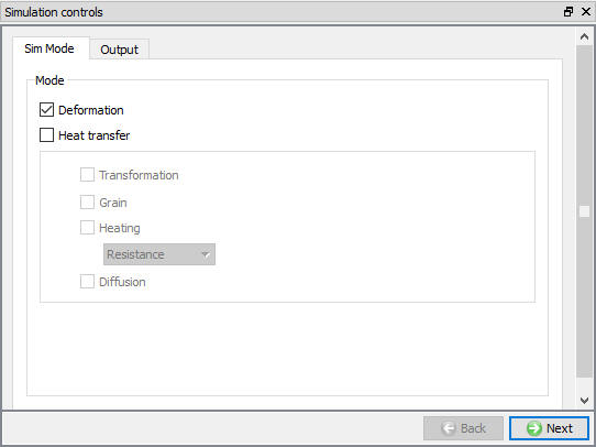
Simulation control window
Material List
In Material list window, click on load material data from Library ![]() option and Load the ‘AISI-4120 ‘ Material from Steel category as shown in Fig. 3DL5.2. Click
option and Load the ‘AISI-4120 ‘ Material from Steel category as shown in Fig. 3DL5.2. Click ![]() until Object page.
until Object page.
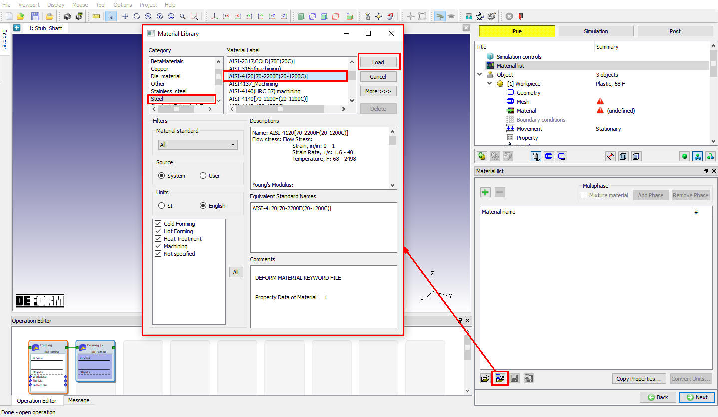
Material List window
Adding objects
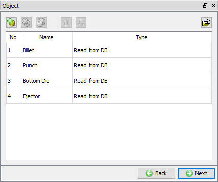
If there aren’t already four objects, add the four objects by clicking the object button ![]() button (see Fig. 3DL5.3.), then click on
button (see Fig. 3DL5.3.), then click on ![]() .
.
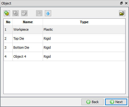
Adding Object Window
Workpiece
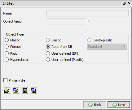
In Workpiece window, change the Object name to Billet and select Object type as Plastic as shown in Fig. 3DL5.4. Click ![]() to geometry page.
to geometry page.
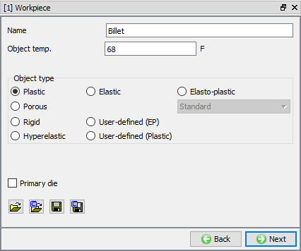
Billet object Window
Billet Geometry
In the Geometry page, select ![]() and define a cylinder that has a Diameter of0.8 ” and a height of 2.7 ” (see Fig. 3DL5.5.). Click on
and define a cylinder that has a Diameter of0.8 ” and a height of 2.7 ” (see Fig. 3DL5.5.). Click on ![]() button. Check geometry and click
button. Check geometry and click ![]() till mesh page.
till mesh page.
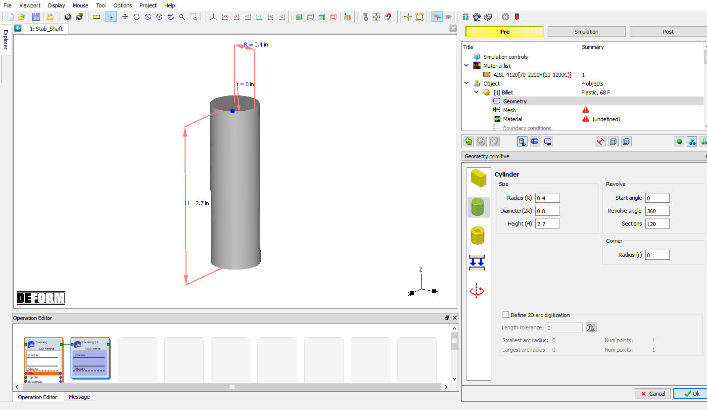
Defining the Workpiece Geometry
Mesh generation
The default settings are adequate for generating a mesh. Click on ![]() to generate the mesh. (see Fig. 3DL5.6.) Click
to generate the mesh. (see Fig. 3DL5.6.) Click ![]() .
.
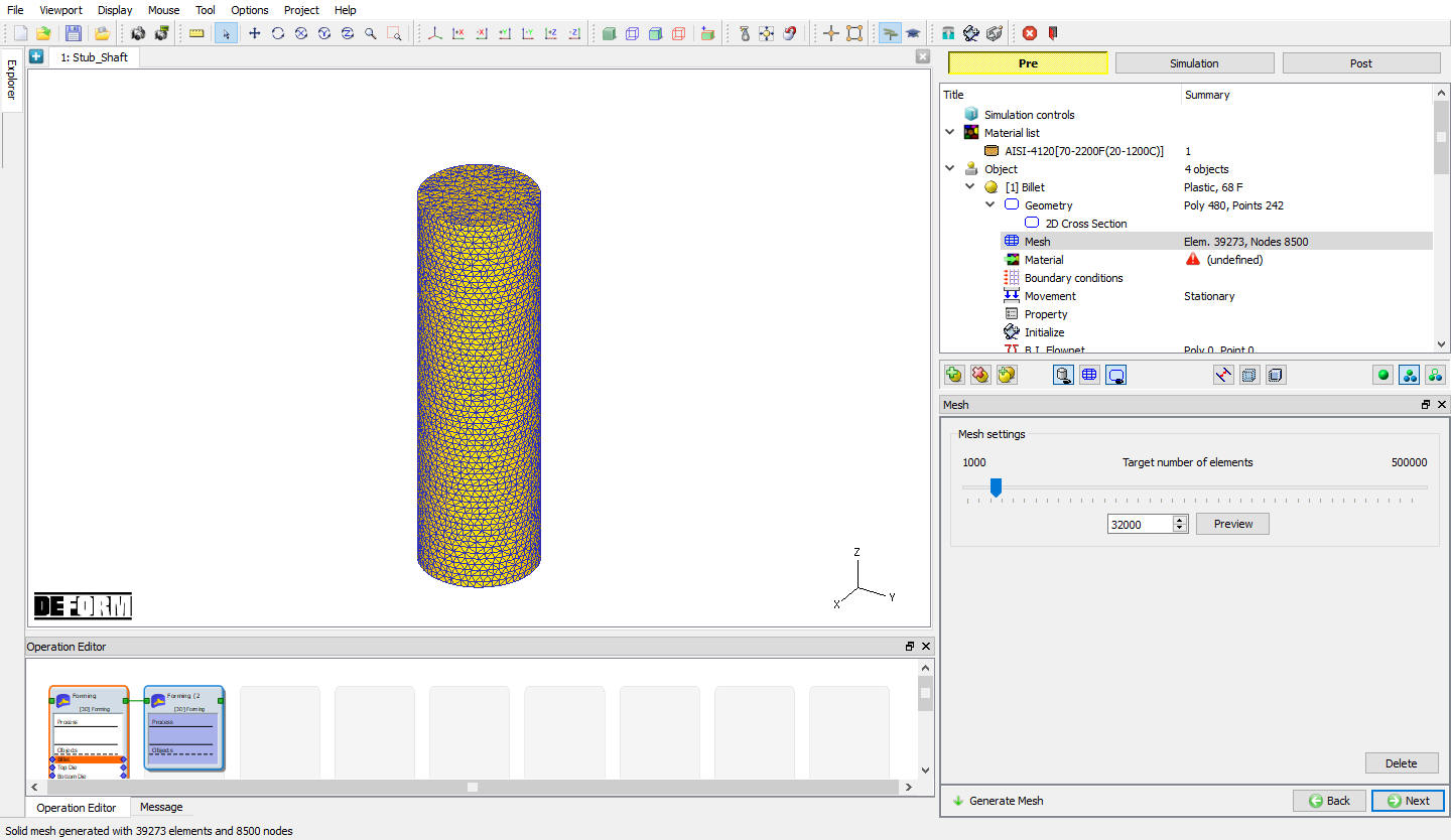
Workpiece Mesh generation
Assigning Billet Material
To assign material for workpiece select the material AISI-4120 from material window. This can be done as shown in below Fig. 3DL5.7. Click ![]() until Top die page.
until Top die page.
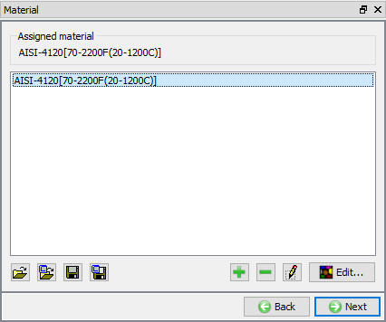
Material selection window
Top Die Definition
In Top Die page, change the name of the top die to Punch , Click ![]() to geometry page.
to geometry page.
Import Punch geometry
Import StubShaft_ConePunch.STL file using Load Geometry from Library ![]() button as shown in Fig. 3DL5.8. Check geometry and click
button as shown in Fig. 3DL5.8. Check geometry and click ![]() until movement page.
until movement page.
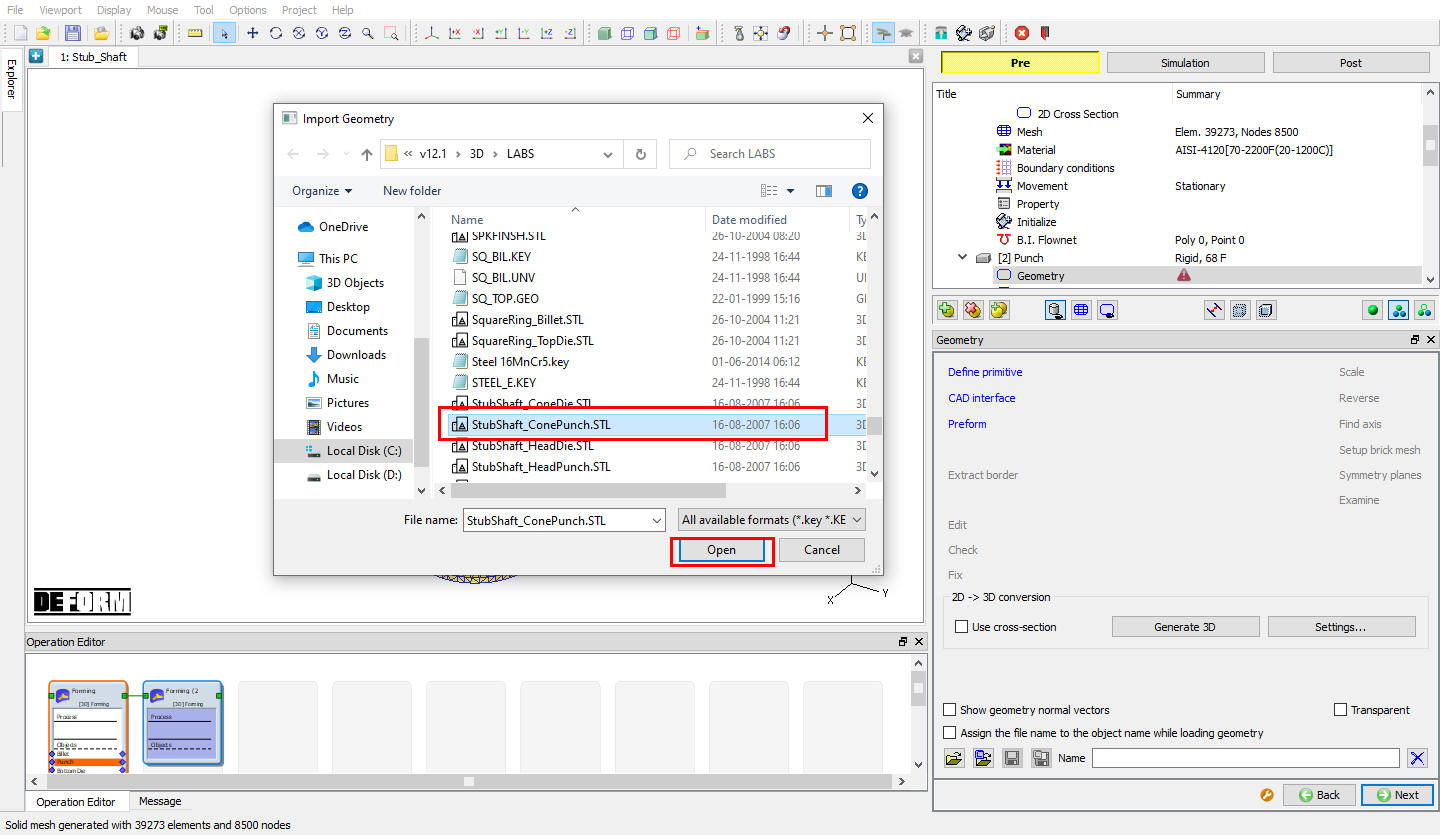
Importing Punch Geometry
Assign Movement to Top Die
Define a speed of 10 in/sec in -Z direction for this lab. Then click ![]() until Bottom Die page.
until Bottom Die page.
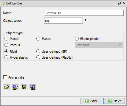
Bottom Die Definition
In Bottom die page, accept the Object type as Rigid and click ![]() (see Fig. 3DL5.9.).
(see Fig. 3DL5.9.).
Bottom Die page
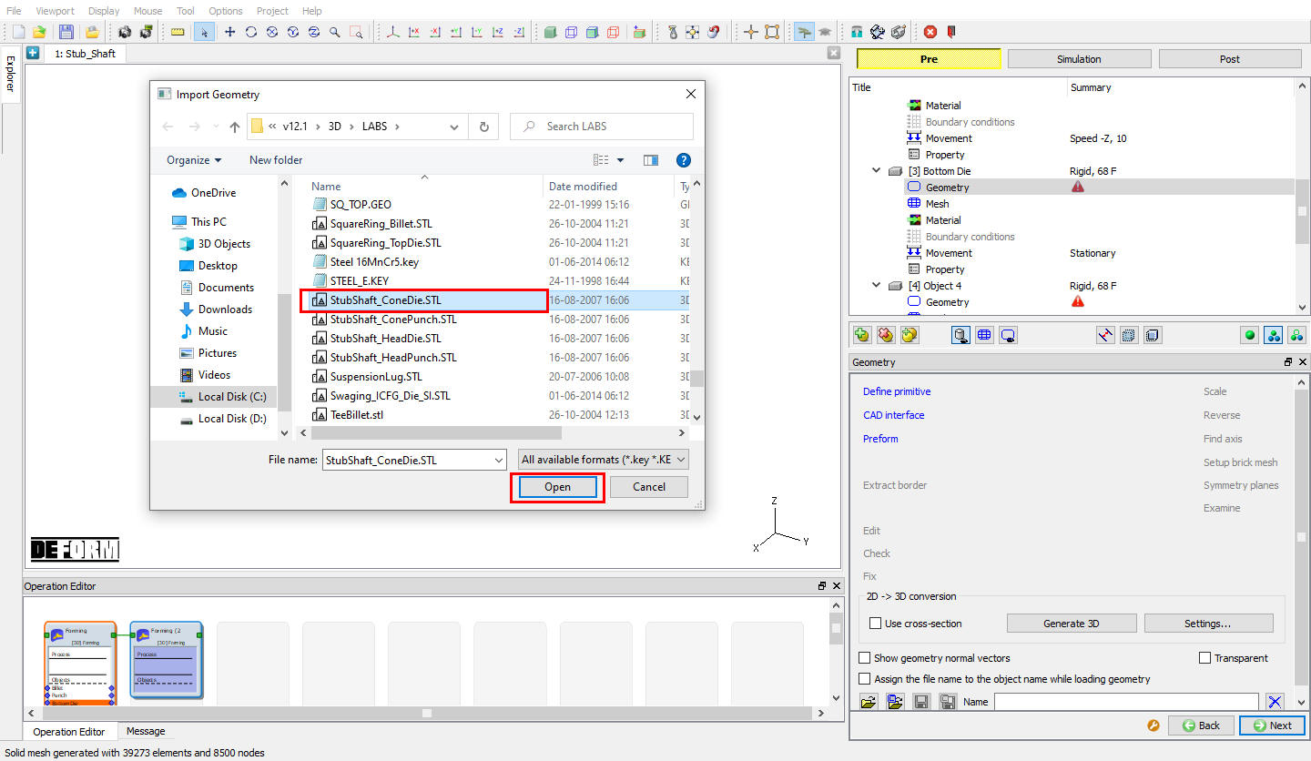
Import Bottom Die Geometry
Import StubShaft_ConeDie.STL file using Load geometry from Library ![]() button as shown in Fig. 3DL5.10. Check geometry and click
button as shown in Fig. 3DL5.10. Check geometry and click ![]() until Object 4 page.
until Object 4 page.
Importing Bottom Die geometry
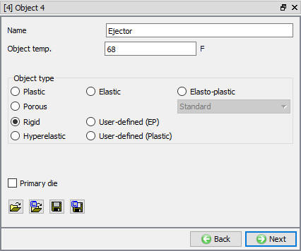
Ejector Definition
In object 4 window, change the Object 4 Name to Ejector and accept the Object type as Rigid as shown in Fig. 3DL5.11., Click ![]() .
.
Ejector object window
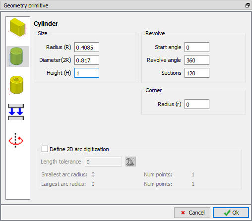
Ejector Geometry
In Ejector geometry window, select and define a cylinder that has a Diameter of 0.817 ” and a height of 1 ” (see Fig. 3DL5.12.), click on ![]() button. Check geometry and click
button. Check geometry and click ![]() until Positioning page.
until Positioning page.
Ejector Geometry Definition
Positioning
Click on ![]() and select
and select ![]() radio button. Change the Positioning Object to the Ejector and the Reference to the Billet. Change the Approach Direction to Z , Press
radio button. Change the Positioning Object to the Ejector and the Reference to the Billet. Change the Approach Direction to Z , Press ![]() (see Fig. 3DL5.13.) and then click
(see Fig. 3DL5.13.) and then click ![]() . click
. click ![]() until Contact page.
until Contact page.
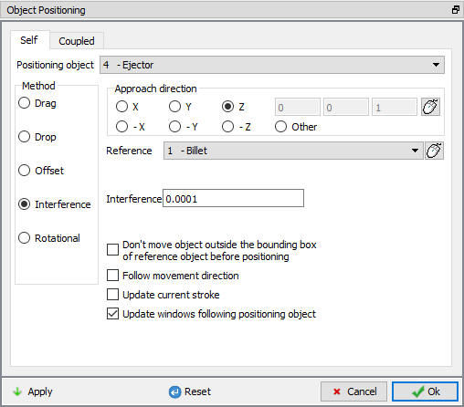
Object Positioning window
Contact Generation
Select user type contact and click on ![]() button. It will add the relationship between the Billet, Punch, Bottom Die and Ejector as shown in Fig. 3DL5.14. As the Dies are Rigid and Billet is plastic, Punch, Bottom Die and Ejector are considered as Master and Billet as Slave.
button. It will add the relationship between the Billet, Punch, Bottom Die and Ejector as shown in Fig. 3DL5.14. As the Dies are Rigid and Billet is plastic, Punch, Bottom Die and Ejector are considered as Master and Billet as Slave.
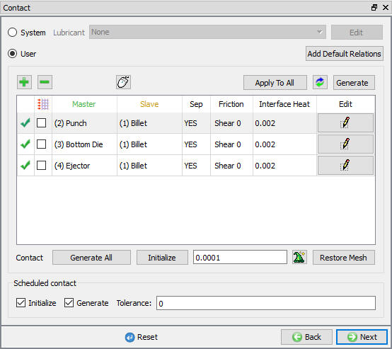
Contact Generation page
Highlight thePunch – Billet relationship and click the ![]() button to modify the contact conditions. In the friction section of the screen (see Fig. 3DL5.15.), there is a pull-down menu that allows the user to choose the appropriate friction conditions of common forming processes.
button to modify the contact conditions. In the friction section of the screen (see Fig. 3DL5.15.), there is a pull-down menu that allows the user to choose the appropriate friction conditions of common forming processes.
Since this simulation takes place at room temperature and the dies are steel, use the pull down menu and select Cold forming (steel dies) from the list. A friction value of 0.12 will automatically be selected.
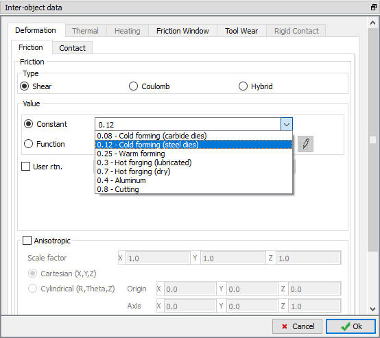
Inter-Object data definition window
Click ![]() to go back to contact window, Since the friction conditions are the same for all the object pairs, the
to go back to contact window, Since the friction conditions are the same for all the object pairs, the ![]() button can be used to copy the interface properties from the first relationship to all of the others. After this is done, all relationships will have a friction of 0.12 defined. Use
button can be used to copy the interface properties from the first relationship to all of the others. After this is done, all relationships will have a friction of 0.12 defined. Use ![]() icon to determine a suitable contact tolerance (a value of about 0.001” will be calculated), then click
icon to determine a suitable contact tolerance (a value of about 0.001” will be calculated), then click ![]() button to generate contact. Switch to Message tab or Observe status bar to know about the contacts generated. Click
button to generate contact. Switch to Message tab or Observe status bar to know about the contacts generated. Click ![]() .
.
Stopping Controls
We want to stop the simulation when the punch and die are within 0.025” of one another. In the Stopping Controls screen, check theDistance between objects option and then click points on the bottom of the Punch and on the top of the Bottom Die. Set the value for this distance to 0.025 ” in theZ direction.(see Fig. 3DL5.16.)
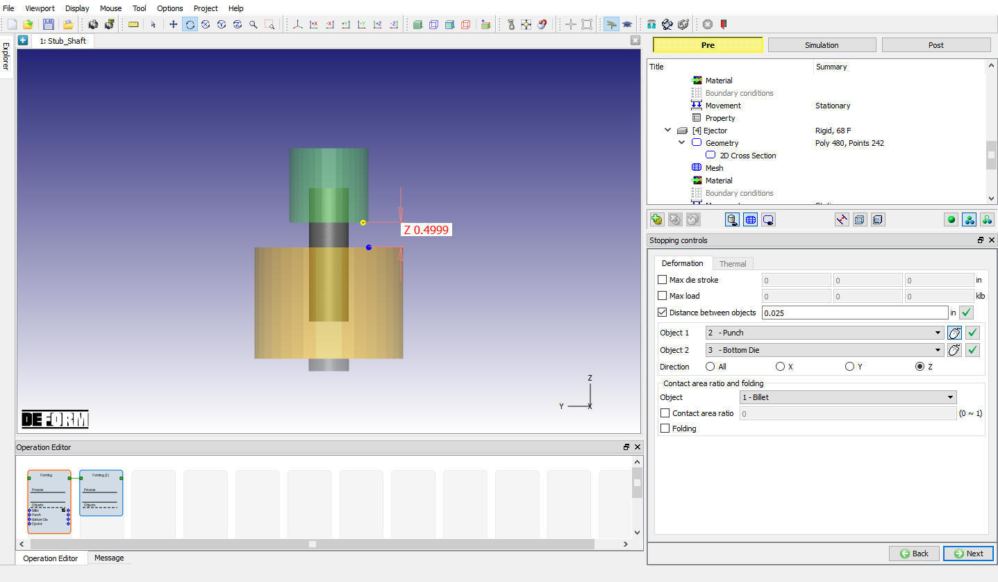
Stopping Controls window
Step Controls
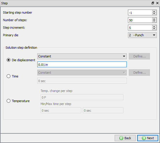
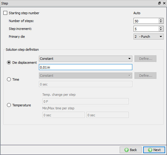
We want the punch to travel 0.5” in 50 steps, so each step will be 0.5/50 or 0.01”. In the Step Controls, under the Solution Steps Definition define the Die Displacement as 0.01 ”. Set the Number of Simulation Steps to 50 and Step Increment to Save to 5. Set the Punch as Primary Die if not selected automatically (see Fig. 3DL5.17.) Click ![]() .
.
Step Controls window
Generate Database
In Generate DB page. Click the ![]() button to have the program check to see if anything was missed in the problem setup. During the checking process:
button to have the program check to see if anything was missed in the problem setup. During the checking process:
Messages in the red color signify data that needs to be fixed before a simulation can be run (such as when you forget to define any material data).
Click on ![]() button to generate the database. When the program is done writing the database, click on
button to generate the database. When the program is done writing the database, click on ![]() tab to go to Next operation.
tab to go to Next operation.
Operation2: Head operation
Simulation Controls
In Simulation controls, uncheck the Heattransfer mode check box. Then click ![]() until Objects page.
until Objects page.
Adding objects
If there aren’t already four objects, add the four objects by clicking the insert object ![]() button (see Fig. 3DL5.18.), then click
button (see Fig. 3DL5.18.), then click ![]() .
.
Adding Object Window
Workpiece Definition
We want to use the workpiece of previous operation last step so, we will make the Workpiece object as Read from DB. Select the Read from DB radio button in Workpiece page. Click ![]() until Top Die (Punch) page. (see Fig. 3DL5.19.)
until Top Die (Punch) page. (see Fig. 3DL5.19.)
Workpiece object page
Top Die Definition
In Top Die (Punch) page, change the Object type to Rigid. If the object name isn’t Punch change it to Punch, Click ![]() .
.
Import Punch geometry:
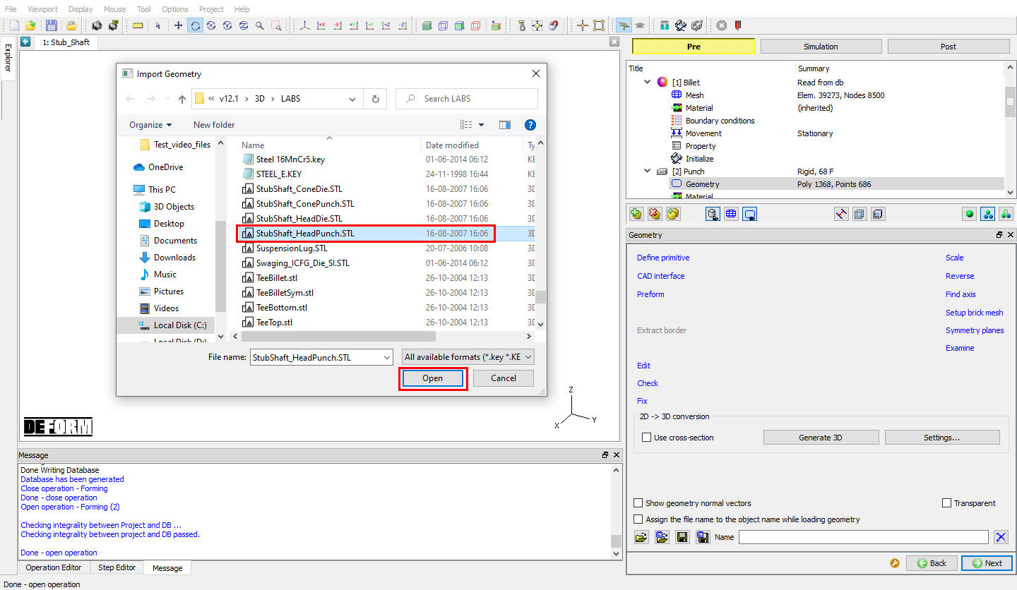
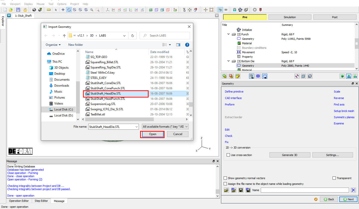
Import StubShaft_HeadPunch.STL file using Load Geometry from Library ![]() button as shown in Fig. 3DL5.20. Check geometry and click
button as shown in Fig. 3DL5.20. Check geometry and click ![]() until movement page.
until movement page.
Loading Punch geometry
Assign Movement to Punch
Define a speed of 10 in/sec in -Z direction for this lab. Then click ![]() until Bottom Die page.
until Bottom Die page.
Bottom Die Definition
In the Bottom die page change the Object type to Rigid and click ![]() .
.
Import Bottom Die Geometry
Import StubShaft_HeadDie.STL file using Load Geometry from Library ![]() button. Check geometry and click
button. Check geometry and click ![]() until object4 (Ejector) page.
until object4 (Ejector) page.
Loading Bottom Die Geometry
Ejector Definition
We will make the Ejector object as Read form DB. Select the Read from DB radio button in Ejector page. Click ![]() until Positioning page.
until Positioning page.
Positioning
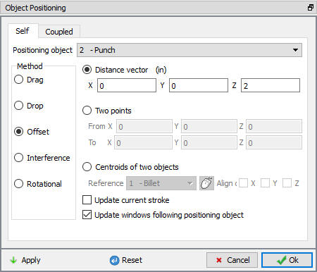
Click on ![]() and change the Positioning Object to the Punch. Select
and change the Positioning Object to the Punch. Select ![]() radio button and position (x=0, y=0 and Z =2) towards Z direction and click
radio button and position (x=0, y=0 and Z =2) towards Z direction and click ![]() (see Fig. 3DL5.22.) and click
(see Fig. 3DL5.22.) and click ![]() . Click
. Click ![]() .
.
Object Positioning window
Scheduled Positioning
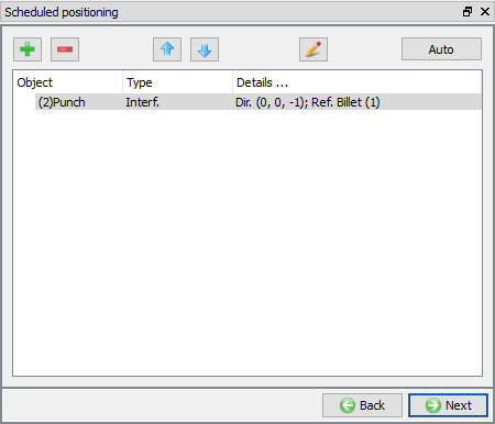
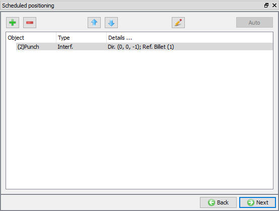
Using Interference positioning we are positioning the Punch to the Workpiece. In Scheduled positioning page, Click on ![]() button and select
button and select ![]() radio button. Change the Positioning Object to the Punch and the Reference to the Billet. Change the Approach Direction to -Z and then click
radio button. Change the Positioning Object to the Punch and the Reference to the Billet. Change the Approach Direction to -Z and then click ![]() . (see Fig. 3DL5.23.) Click
. (see Fig. 3DL5.23.) Click ![]() .
.
Scheduled Positioning window
Contact Generation
Define the contact relations using the same settings which we defined for the first operation in the section 5.1.11. Click ![]() .
.
Stop Controls
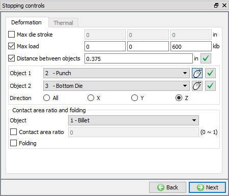
Turn on the Distance between objects option and define the reference points as shown in the Fig. 3DL5.24. Set the stopping distance as 0.375 ” in Z direction.
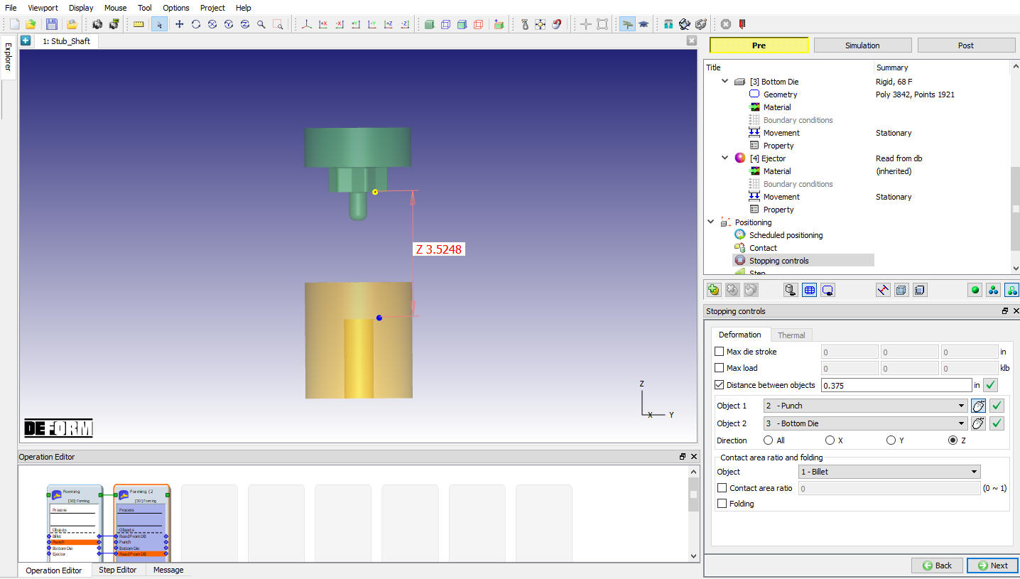
Distance Between Objects stopping control
We will also specify a maximumload for this part. Under the Deformation tab, set the Max load to X = 0, Y =0 and Z= 600. Now if the press load exceeds 600 Klb(300Tons), the simulation will stop, even if the distance between tools has not been reached (see Fig. 3DL5.25.). Click ![]() .
.
Stop controls page
Step Controls
Estimate the total punch travel, which will be roughly 1.5”. At the end of the simulation we want a gap of 0.375. It’s ok if we overshoot the die travel by a little bit here because we will set a stopping condition to make sure that the tools stop when they are 0.375’’ apart. So we will only subtract 0.3 from 1.5. This will give us a total punch travel of 1.2. For 100 steps, that means that the punch needs to travel 0.012’’ every step.
Set the Number of Simulation Steps to 100 , step increment to save to 5 and constant die displacement as 0.012 ‘’. (see Fig. 3DL5.26.) Click ![]() .
.
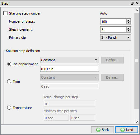
Step Controls window
Generate Database
See the Status in Generate DB page, if we see Input error, check the data missing and complete it, for this lab sequence expect “DB generation is not required for this operation. It will occur at run time.” message
Save the project and click on ![]() mode to run the simulation.
mode to run the simulation.
Running simulation
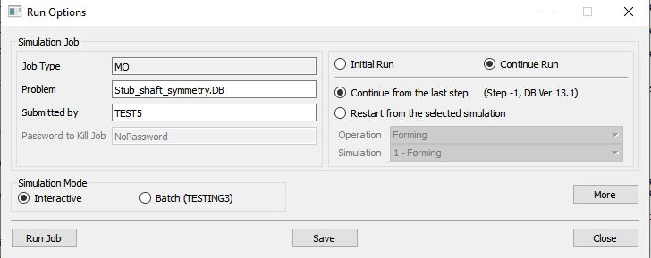
Click on the ![]() action label under the simulation tab (See Fig. 3DL5.27.), Run Options dialog will open as shown in Fig. 3DL5.28. Use the default Continue Run option to select “Continue from the last step ” option and then select the Simulation mode as Interactive and click on
action label under the simulation tab (See Fig. 3DL5.27.), Run Options dialog will open as shown in Fig. 3DL5.28. Use the default Continue Run option to select “Continue from the last step ” option and then select the Simulation mode as Interactive and click on ![]() button to run the simulation.
button to run the simulation.

Simulation Options
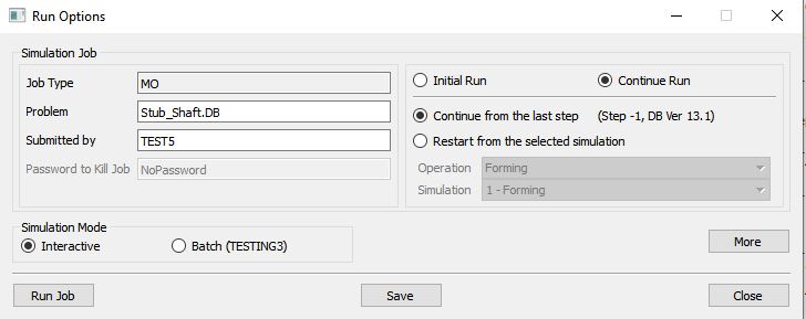
Run Simulation window
The progress of the simulation can be monitored as it is running by looking at the Simulation Message tab and Simulation Graphics from the Graphics display region in Simulation mode. As long as the ![]() option is checked in Simulation Message tab, which is the default setting, the Message file will refresh automatically.
option is checked in Simulation Message tab, which is the default setting, the Message file will refresh automatically.
The Message file provides information about which simulation step the simulation is currently on and also gives information dealing with how well the simulation is running.
When the simulation is finished without any issues, check the messages in LOG file, when all operation completes we will see messages in LOG file:”MULTIPLE OPERATION COMPLETED”.
Post process the results
After the simulation is completed, Switch to ![]() tab.
tab.
Play through results
Use the ![]() function to play through both the cone blow and the heading blow.
function to play through both the cone blow and the heading blow.
Experiment with different part shading options.
Finding folds
Click on the ![]() button to open the State Variables window.
button to open the State Variables window.
Click on foldingangle and change scaling mode to “User.” Insert values of 270 and 271 for Min and Max respectively. Click on ![]() . (See Fig. 3DL5.29.)
. (See Fig. 3DL5.29.)
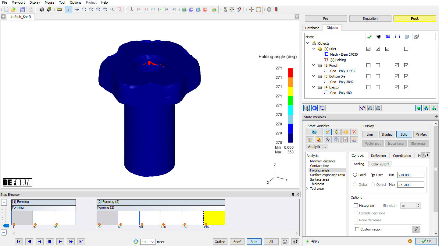
State Variable Window with fold on workpiece
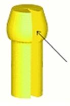
The fold can now be seen in red. User can play through the time steps and see the fold form. User can also right click on the color bar to experiment with different color bar types. (See Fig. 3DL5.30.)
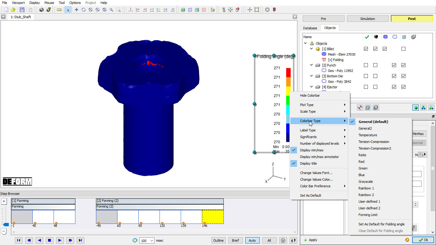
Image showing fold in the workpiece
Use the slicing tool ![]() to cut the piece vertically. Click on the radio button next to “Curve + Plane ” as shown in Fig. 3DL5.31.
to cut the piece vertically. Click on the radio button next to “Curve + Plane ” as shown in Fig. 3DL5.31.
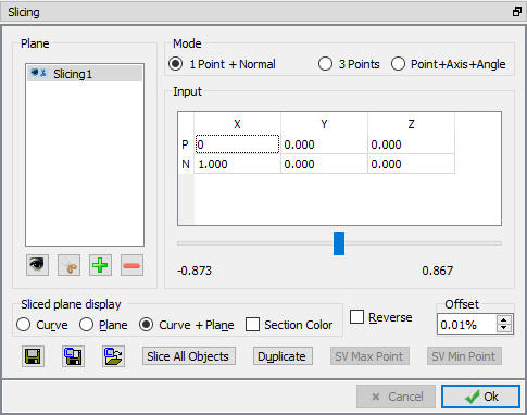
Slicing Window
With this view you can easily see the folds. (See Fig. 3DL5.32.)
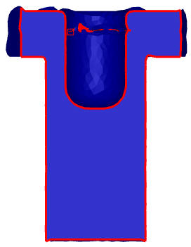
Sliced Object
Determining Fill
Press clear ![]() to turn off all the variables. Then turn on show contact nodes
to turn off all the variables. Then turn on show contact nodes ![]() .
.
DEFORM places dots where contact has been made with the tool. Places without dots can represent an under fill situation (see Fig. 3DL5.33.). The fill can also be seen by cutting a section through the part.
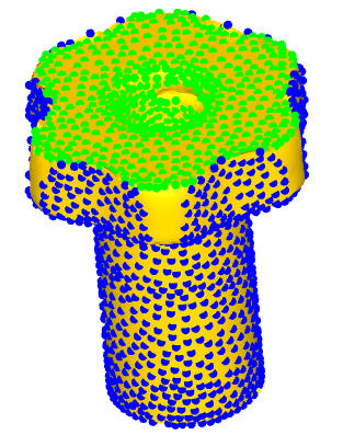
Determining filling in the object
Turn off contact ![]() . Display all the tools and the workpiece
. Display all the tools and the workpiece ![]() .
.
Use the slicing tool to slice the objects about the x-y plane (Make the N direction (0,0,1). Pick “Curve ” under the ‘Sliced plane display’ option. (See Fig. 3DL5.34.)
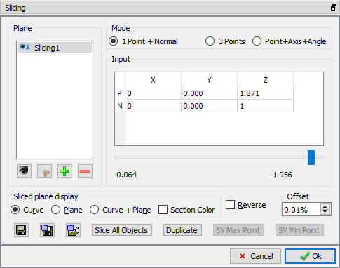
Slicing window
Click on the Z coordinate next to the P (point) input. Then use the slider bar to move the slicing plane up and down the Z axis.
Select “+ Z direction” button to view the objects from the +Z direction as shown in Fig. 3DL5.35.
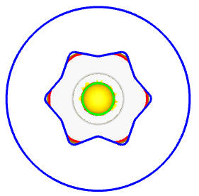
Object in +Z view
User can directly see the gap between the tool and the workpiece. Delete ![]() the slicing plane from the slicing menu.
the slicing plane from the slicing menu.
So far we have used qualitative methods to see under fill. User can also plot the distance between the workpiece and the tooling.
Click on State Variables ![]() Icon. Select “Minimumdistance ” and press
Icon. Select “Minimumdistance ” and press ![]() .
.
Turn off all the tools and display just the workpiece ![]() . The normal distance between the workpiece and the closest tool will be displayed. User can left mouse click anywhere on the part. This will plot the minimum distance value on the color bar. (See Fig. 3DL5.36.)
. The normal distance between the workpiece and the closest tool will be displayed. User can left mouse click anywhere on the part. This will plot the minimum distance value on the color bar. (See Fig. 3DL5.36.)
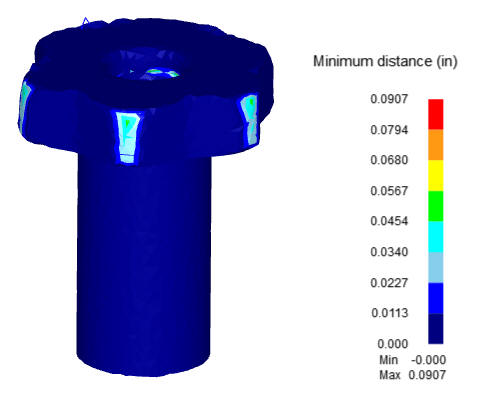
Image Showing Minimum distance region
Symmetry/Thermal Operations
Create a new simulation
Now we are going to perform the Cone_Blow operation, from above, with a heated billet. This involves heating the billet, letting it sit in air for 6 seconds (transfer), letting it sit in the die for 2 seconds (dwell) and then forming it (cone). We will do all of this by simulating 1/12th of the part using symmetry as shown in Fig. 3DL5.37.

Workpiece showing 1/12th of the symmetry
Create a new problem either by selecting File![]() **New Problem** or by clicking the NewProblem
**New Problem** or by clicking the NewProblem![]() icon. The Problem Setup window will appear. Select “Integrated Manufacturing Process “ radio button and units system as “English “ radio button in units field. Define Problem Name as “**Stub_shaft_symmetry** “ and make sure the “Show option dialog ” check box is turned on (if we do not turn on the “Show option dialog” check box, then we will not get the New Project dialog). Then click on
icon. The Problem Setup window will appear. Select “Integrated Manufacturing Process “ radio button and units system as “English “ radio button in units field. Define Problem Name as “**Stub_shaft_symmetry** “ and make sure the “Show option dialog ” check box is turned on (if we do not turn on the “Show option dialog” check box, then we will not get the New Project dialog). Then click on ![]() button to open a new problem using the Deform Integrated Manufacturing Process.
button to open a new problem using the Deform Integrated Manufacturing Process.
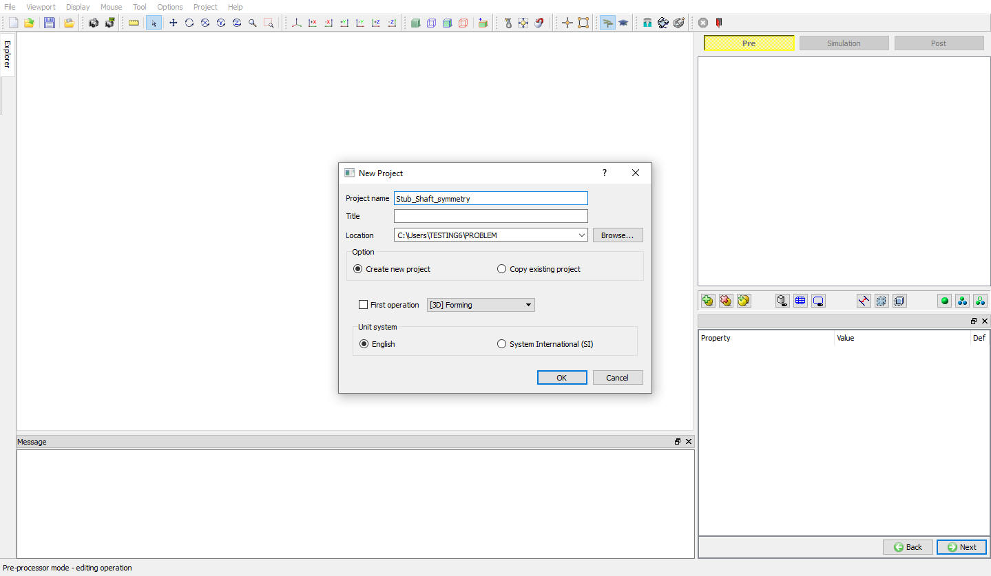
Problem defining window
MO wizard will open along with project naming window as shown in Fig. 3DL5.38. In the field of project name. In the field of project name, set the project name as ‘Stub_shaft_symmetry ‘ and click ![]() .
.
Add operations
Add two 3D Heat Transfer operations and one 3D Forming operations from Operation list in Explorer. Operation can be add by clicking on ![]() button next to respective operation or user can also add the operation by dragging and dropping the operation into Operation Editor region.
button next to respective operation or user can also add the operation by dragging and dropping the operation into Operation Editor region.
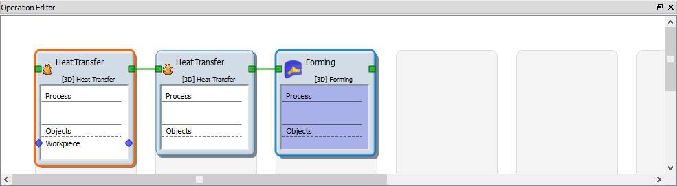
Adding operations
Importing the DB
After adding all three operations, import previously simulated Stub_Shaft.DB , select the firststep and click ![]() .
.
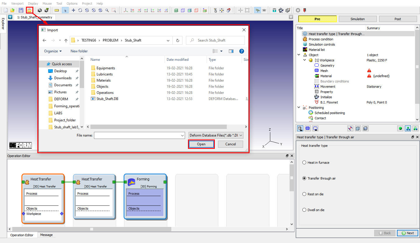
Importing DB
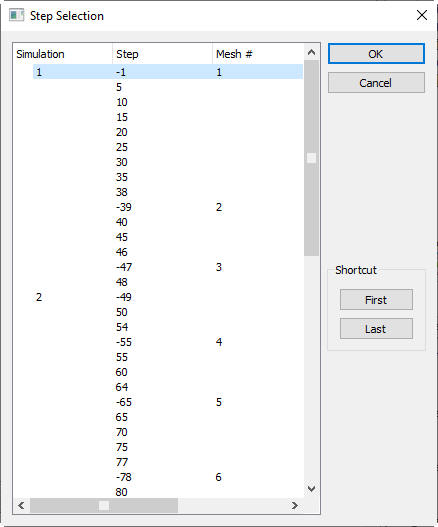
Step selection window
Selecting Heat Transfer Type
Select Transfer through air heat transfer type for first operation as shown in Fig. 3DL5.42. This will set the default heat transfer settings for heating operation. Click ![]() to continue.
to continue.
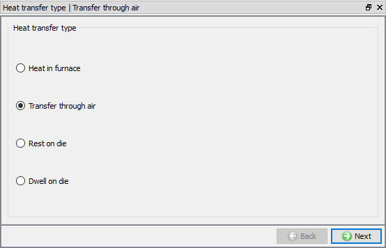
Heat transfer type selection for Furnace Heating operation
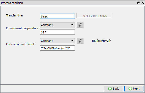
Set Process Conditions
Define Heatingtime as 6 sec at 68°F furnace temperature or environment temperature as shown in Fig. 3DL5.43. and click ![]() to continue.
to continue.
Process condition window
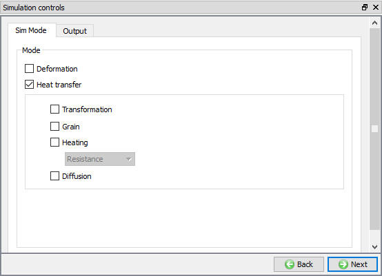
Select Simulation Controls
Keep onlyHeat Transfer mode checked as only heat transfer is modelling as shown in Fig. 3DL5.44. and click ![]() .
.
Simulation Controls settings for Furnace Heating
Material page
Delete the importedAISI-4120[70-2200F(20-1200C)] material from the list.
Objects page
In objects page we are seeing all the objects imported from the stubshaft DB.
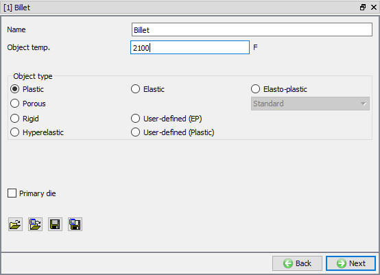
Defining Billet
In Billet object window accept the objecttype as ‘Plastic ’ and change the objecttemperature to 2100 °F. (See Fig. 3DL5.45.) Click on ![]() .
.
Billet Definition Page
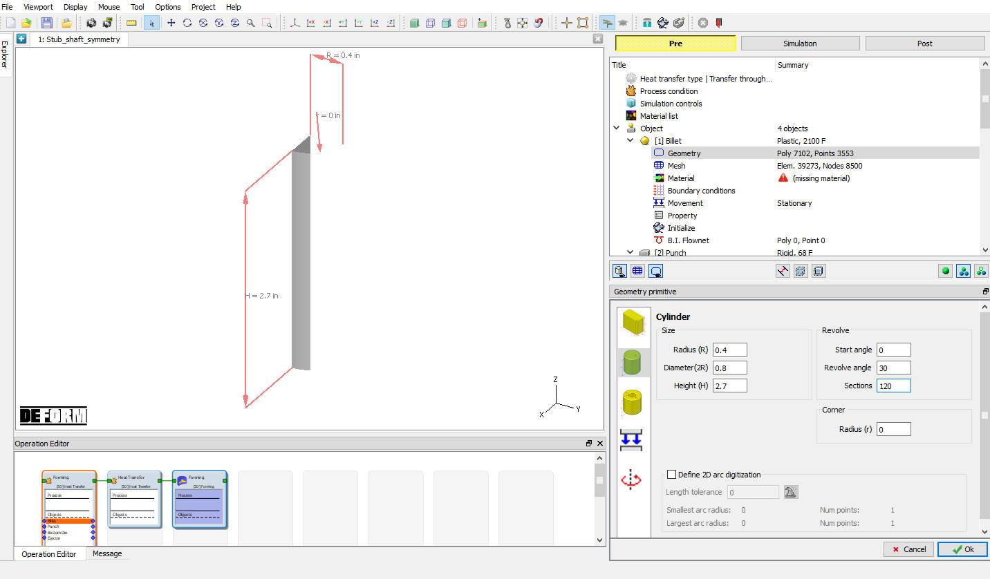
Billet Geometry
In the Geometry page, select and define a cylinder that has a Diameter of 0.8 ”, height of 2.7 ” and Revolveangle as 30 deg (see Fig. 3DL5.46.). Click on ![]() button. Check geometry and define the planar symmetry for the two symmetry surfaces (see Fig. 3DL5.47. and Fig. 3DL5.48.). Click
button. Check geometry and define the planar symmetry for the two symmetry surfaces (see Fig. 3DL5.47. and Fig. 3DL5.48.). Click ![]() until mesh page.
until mesh page.
Defining the Workpiece Geometry
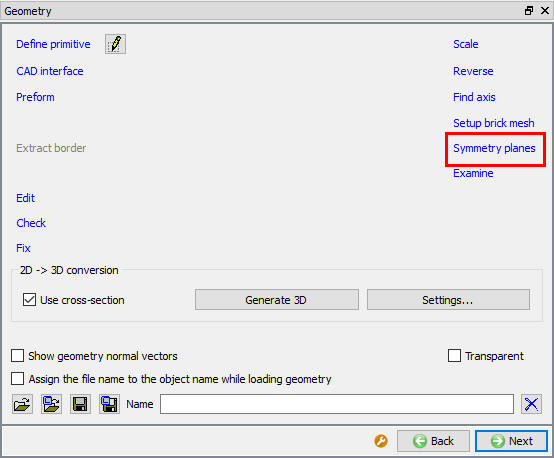
Geometry page
Planar symmetry definition
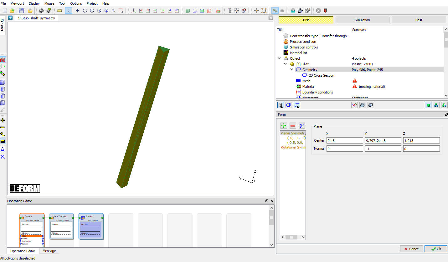
Generate Mesh
Generate the mesh using 32000 elements (see Fig. 3DL5.49.). Complete range of meshing options are also available in expert mode (![]() ), if user needs to have more control on the mesh generated. Click on
), if user needs to have more control on the mesh generated. Click on ![]() to continue.
to continue.
Mesh generation window
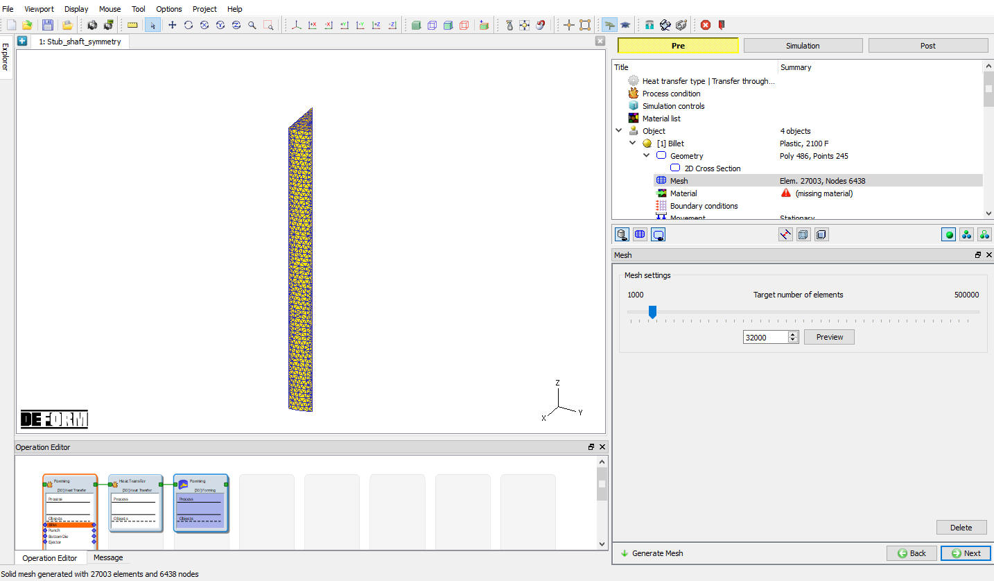
Assign Workpiece Material
Using Load from library ![]() option, load AISI-8620 material from Steel category, to assign material for workpiece select the material ‘AISI-8620 ’ from material window. This can be done as shown in Fig. 3DL5.50. Click on
option, load AISI-8620 material from Steel category, to assign material for workpiece select the material ‘AISI-8620 ’ from material window. This can be done as shown in Fig. 3DL5.50. Click on ![]() to continue.
to continue.
Object material selection window
Defining Boundary Conditions
In BCC page, check the default assigned Heat exchange with Environment BCC to the entire outer surface of the Billet except symmetry surfaces. Click ![]() until Punch Movement page.
until Punch Movement page.
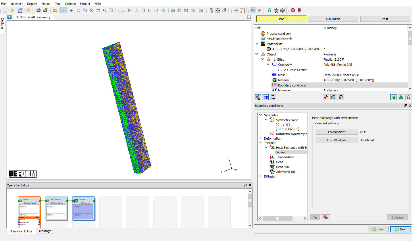
BCC Definition window
Punch Movement Definition
In Punch movement page, Change the “constant value” velocity to 0. Click ![]() until Positioning page.
until Positioning page.
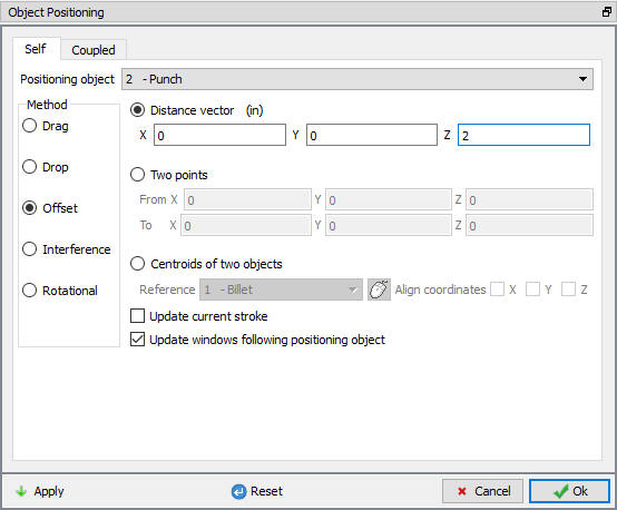
Positioning
We will move the tools away from the object so they will not interfere with the cooling process. Click on the ![]() button to open the positioning page. Use
button to open the positioning page. Use ![]() to move the Punch2 inches in the “Z ” direction. Also move the Bottomdie and Ejector -2 inches in the “Z ” direction. Press
to move the Punch2 inches in the “Z ” direction. Also move the Bottomdie and Ejector -2 inches in the “Z ” direction. Press ![]() to exit the positioning menu. (See Fig. 3DL5.52.) Click
to exit the positioning menu. (See Fig. 3DL5.52.) Click ![]() until Step controls window
until Step controls window
Objects positioning window
Define Step Controls
Set the Number of simulation steps as 50 at 0.12 sec each and saving every5 steps (see Fig. 3DL5.53.). Advanced Simulation controls settings are available in expert mode (![]() ). Click
). Click ![]() to proceed to the database generation stage.
to proceed to the database generation stage.
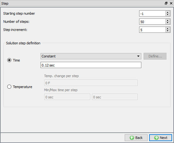
Simulation controls settings for furnace heating operation
Generate Database
In Generate DB page. Click the ![]() button to have the program check to see if anything was missed in the problem setup. During the checking process:
button to have the program check to see if anything was missed in the problem setup. During the checking process:
Messages in the red color signify data that needs to be fixed before a simulation can be run (such as when you forget to define any material data).
Click on ![]() button to generate the database. When the program is done writing the database, click on
button to generate the database. When the program is done writing the database, click on ![]() tab to go to Next operation.
tab to go to Next operation.
Selecting Heat Transfer Type (2nd Operation)
Select Rest on die heat transfer type for second operation as shown in Fig. 3DL5.54. This will set the default heat transfer settings for heating operation. Click ![]() to continue.
to continue.
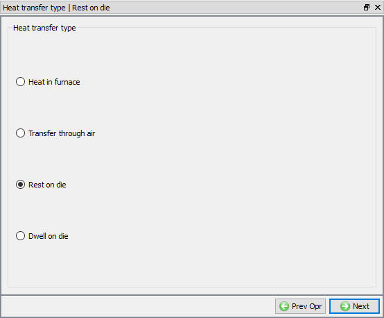
Heat transfer type selection for Furnace Heating operation
Set Process Conditions
Define Resting time as 2 sec at 68 °F furnace temperature or environment temperature as shown in Fig. 3DL5.55. and click ![]() to continue.
to continue.
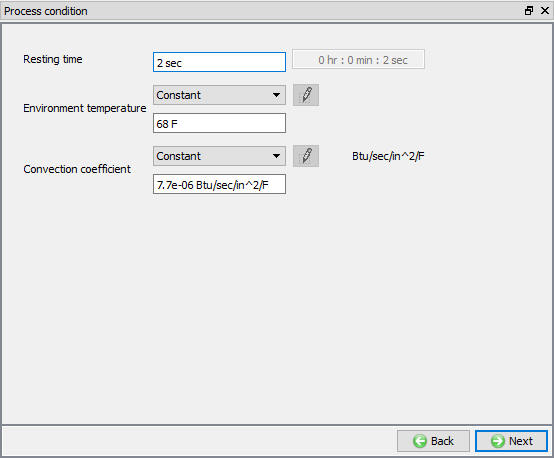
Process condition window
Select Simulation Controls
Keep only Heat Transfer mode checked as only heat transfer is modelling as shown in Fig. 3DL5.56. and click ![]() until objects page.
until objects page.
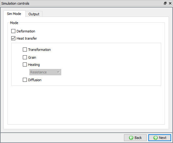
Simulation Controls settings for Furnace Heating
Defining the objects
When we enter the second operation we are seeing all the objects as Read from DB, accept all the objects as Read from DB objects (see Fig. 3DL5.57.). Click ![]() until Scheduled Positioning page.
until Scheduled Positioning page.
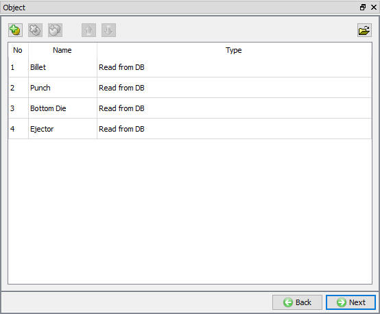
Objects page
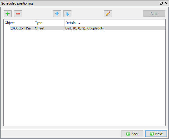
Scheduled Positioning
Use ![]() Positioning option to move the Bottom die and Ejector 2 inches in the “Z ” direction (see Fig. 3DL5.58.). Click
Positioning option to move the Bottom die and Ejector 2 inches in the “Z ” direction (see Fig. 3DL5.58.). Click ![]() .
.
Scheduled Positioning
Contact Generation
Select user type contact and click on ![]() (Add relationship) button twice and select Bottomdie as Master and Billet as Slave for first relation and for second relation select Ejector as Master and Billet as Slave as shown in Fig. 3DL5.59.
(Add relationship) button twice and select Bottomdie as Master and Billet as Slave for first relation and for second relation select Ejector as Master and Billet as Slave as shown in Fig. 3DL5.59.
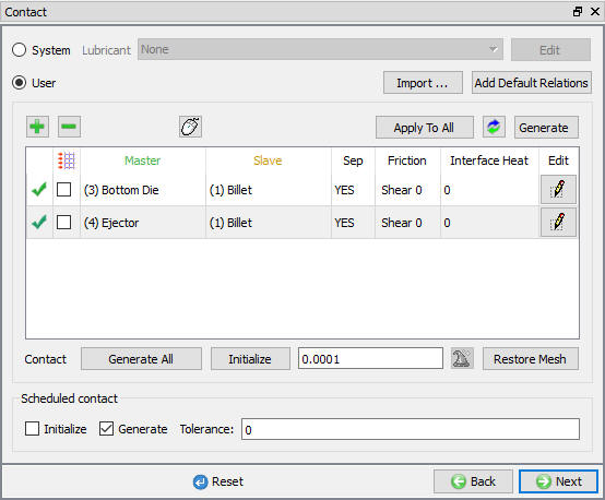
Inter-object relationship between workpiece and bottom die
Click on ![]() (Edit) relationship button and select the pull down option “Free Resting “ in the thermal section to define the inter-object heat transfer coefficient as shown in Fig. 3DL5.60. Click
(Edit) relationship button and select the pull down option “Free Resting “ in the thermal section to define the inter-object heat transfer coefficient as shown in Fig. 3DL5.60. Click ![]() to close the Editing window. It will generate the inter-object contact at the beginning of the resting operation while simulating. Click
to close the Editing window. It will generate the inter-object contact at the beginning of the resting operation while simulating. Click ![]() until step controls window.
until step controls window.
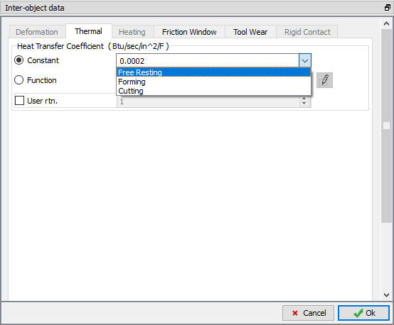
Inter-object Heat transfer coefficient selection for resting
Define Step Controls
Set the number of simulation steps as 20 at 0.1 sec each and saving every5 steps (see Fig. 3DL5.61.). Advanced Simulation controls settings are available in expert mode (![]() ). Click
). Click ![]() to proceed to the database generation stage.
to proceed to the database generation stage.
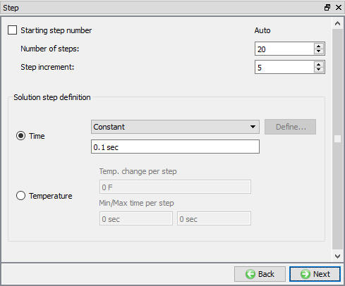
Simulation controls settings for furnace heating operation
Generate Database
See the Status in Generate DB page, if we see Input error, check the data missing and complete it, for this lab sequence expect “DB generation is not required for this operation. It will occur at run time.” message. Save the project and click on ![]() .
.
Select Simulation Controls( 3rd Operation)
For the forming operation turnon the Deformation check box along with heattransfer. Click ![]() until objects page.
until objects page.
Defining the objects
If there aren’t already four objects, add the four objects by clicking the insert object ![]() button (see Fig. 3DL5.62.). All four objects should be defined as Read from DB objects. If they aren’t set them that way by visiting every object page.
button (see Fig. 3DL5.62.). All four objects should be defined as Read from DB objects. If they aren’t set them that way by visiting every object page.

Objects page
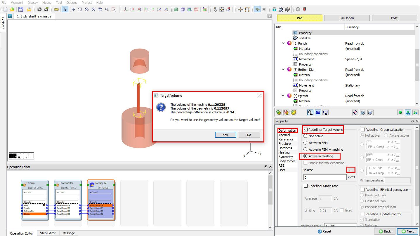
Defining Workpiece
Workpiece Properties :
In Billet Properties page, check “Redefine : Target volume “ check box and select Active in Meshing radio button then click on the ![]() icon. Click
icon. Click ![]() for popup window. (See Fig. 3DL5.63.)
for popup window. (See Fig. 3DL5.63.)
Properties page
Defining the Punch
Defining the Punch movement :
Define a speed of 4 in/sec in -Z direction for the Punch object. Then click on ![]() until Scheduled positioning page.
until Scheduled positioning page.
Scheduled Positioning
In scheduled Positioning page, click on ![]() button and select the ‘Positioning object’ as Punch , method as ‘Interference ’ with respect to ‘Billet ’ in the -Z direction (see Fig. 3DL5.64.). Click
button and select the ‘Positioning object’ as Punch , method as ‘Interference ’ with respect to ‘Billet ’ in the -Z direction (see Fig. 3DL5.64.). Click ![]() to continue.
to continue.
Scheduled Positioning window
Contact Generation
Select user type contact and click on ![]() button. It will add the relationship between the Billet, Punch, Bottom Die and Ejector (see Fig. 3DL5.66.). As the Dies are Rigid and Billet is plastic, Top and Bottom Dies are considered as Master and Billet as Slave.
button. It will add the relationship between the Billet, Punch, Bottom Die and Ejector (see Fig. 3DL5.66.). As the Dies are Rigid and Billet is plastic, Top and Bottom Dies are considered as Master and Billet as Slave.
Highlight the Punch – Billet relationship and click the ![]() button to modify the contact conditions. In the friction section of the screen (see Fig. 3DL5.65.), there is a pull-down menu that allows the user to choose the appropriate friction conditions of common forming processes.
button to modify the contact conditions. In the friction section of the screen (see Fig. 3DL5.65.), there is a pull-down menu that allows the user to choose the appropriate friction conditions of common forming processes.
Since this is hot forming simulation and the dies are steel, use the pull down menu and select Hot forming (lubricated) from the list. A friction value of 0.3 will automatically be selected. Under Thermal tab select “Forming “ from the list, a Heat transfer coeffecient of “ 0.002 “ .
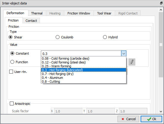
Inter-object friction coefficient definition window
Click ![]() to go back to Contact window, Since the friction conditions are the same for all the object pairs, the
to go back to Contact window, Since the friction conditions are the same for all the object pairs, the ![]() button can be used to copy the interface properties from the first relationship to all of the others. After this is done, all relationships will have a friction of 0.3 defined as shown in Fig. 3DL5.66. Since the contact will initialize and generate while generating database. Click
button can be used to copy the interface properties from the first relationship to all of the others. After this is done, all relationships will have a friction of 0.3 defined as shown in Fig. 3DL5.66. Since the contact will initialize and generate while generating database. Click ![]() to continue.
to continue.
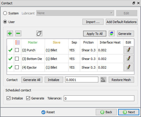
Inter-Object relationship definition for forming operation
Stopping Controls
We want to stop the simulation when the punch and die are within 0.025” of one another. In the Stopping Controls screen, check the Distance between objects option and then click points on the bottom of the punch and on the top of the Bottom Die. Set the value for this distance to 0.025 ” in the Z direction (see Fig. 3DL5.67.). Click ![]() to Step controls page.
to Step controls page.
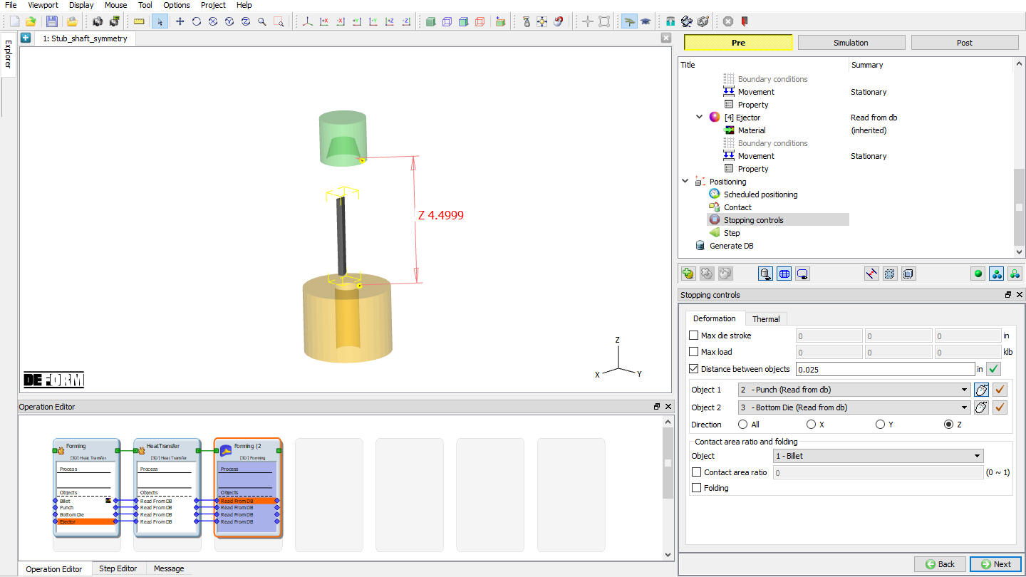
Stopping Controls window
Step Controls
We want the punch to travel 0.5” in 50 steps, so each step will be 0.5/50 or 0.01”. In the Step Controls enter the Solution Steps Definition to be With Equal Die Displacement of 0.01”. Set the Number of Simulation Steps to 50 and Step Increment to Save to 5. Set the Punch as PrimaryDie if not selected automatically (see Fig. 3DL5.68.). Click ![]() to DB generation page.
to DB generation page.
Step Controls window
Generate Database
See the Status in Generate DB page, if we see Input error, check the data missing and complete it, for this lab sequence expect “DB generation is not required for this operation. It will occur at run time.” message.
Save the project and click on ![]() mode to run the simulation.
mode to run the simulation.
Running simulation
Click on ![]() label under the simulation tab (see Fig. 3DL5.70.), as we click on the Run option, use the default Continue Run option to select “Continue from the last step ” option and then select the Simulation mode as Interactive and click on
label under the simulation tab (see Fig. 3DL5.70.), as we click on the Run option, use the default Continue Run option to select “Continue from the last step ” option and then select the Simulation mode as Interactive and click on ![]() button to run the simulation.
button to run the simulation.
Simulation Options
Run Simulation window
The progress of the simulation can be monitored as it is running by looking at the Simulation Message tab and Simulation Graphics from the Graphics display region in Simulation mode. As long as the ![]() option is checked in Simulation Message tab, which is the default setting, the Message file will refresh automatically.
option is checked in Simulation Message tab, which is the default setting, the Message file will refresh automatically.
The Message file provides information about which simulation step the simulation is currently on and also gives information dealing with how well the simulation is running.
When the simulation is finished without any issues, check the messages in LOG file, when all operation completes we will see messages in LOG file:”MULTIPLE OPERATION COMPLETED”.
Post process the results
After the simulation is completed, Switch to ![]() tab.
tab.
Click on ![]() icon, so that only the workpiece is visible. Click Temperature state variable to plot the temperature of the workpiece. Right click on the Temperature scale and Select “Colorbar type ” then “Temperature ”. (See Fig. 3DL5.71.)
icon, so that only the workpiece is visible. Click Temperature state variable to plot the temperature of the workpiece. Right click on the Temperature scale and Select “Colorbar type ” then “Temperature ”. (See Fig. 3DL5.71.)
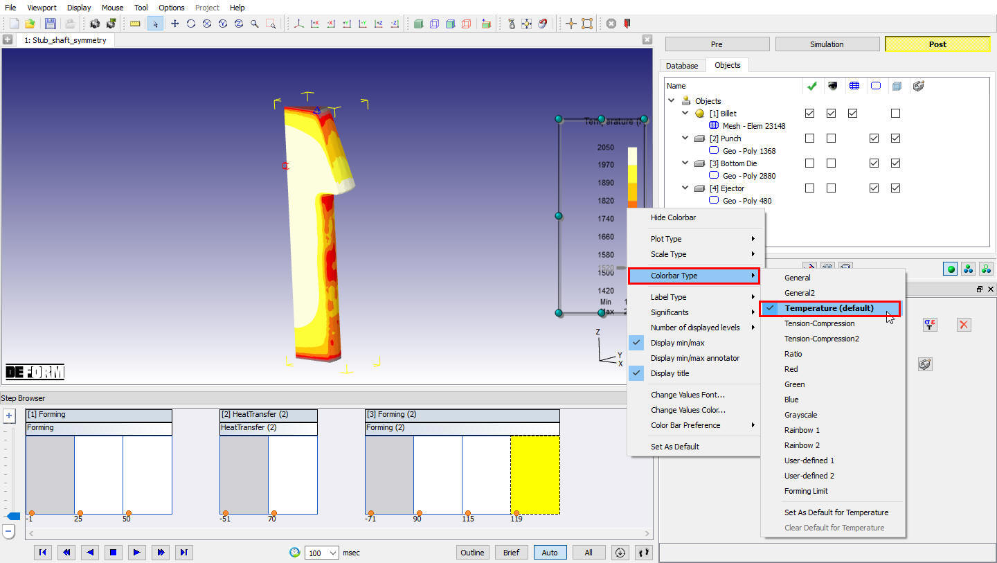
Object showing temperature values with Temperature Color Bar type
Click on Mirror symmetry ![]() icon. Click on the symmetry faces until you can see the whole part. This will take 11 clicks. (See Fig. 3DL5.72.)
icon. Click on the symmetry faces until you can see the whole part. This will take 11 clicks. (See Fig. 3DL5.72.)
Mirroring of symmetric faces
Tool Stress Analysis
Opening project file
Create a new problem either by selecting File![]() **New Problem** or by clicking the NewProblem
**New Problem** or by clicking the NewProblem![]() icon. The Problem Setup window will appear. Select “Integrated Manufacturing Process “ radio button and units system as “English “ radio button in units field. Define Problem Name as “StubShaft_ToolStress “ and make sure the “Show option dialog ” check box is turned on (if we do not turn on the “Show option dialog” check box, then we will not get the New Project dialog). Then click on
icon. The Problem Setup window will appear. Select “Integrated Manufacturing Process “ radio button and units system as “English “ radio button in units field. Define Problem Name as “StubShaft_ToolStress “ and make sure the “Show option dialog ” check box is turned on (if we do not turn on the “Show option dialog” check box, then we will not get the New Project dialog). Then click on ![]() button to open a new problem using the Deform Integrated Manufacturing Process.
button to open a new problem using the Deform Integrated Manufacturing Process.
MO wizard will open along with project naming window. In the field of project name, select the copy existing project radio button. Select the source location browse button and import the Stub_Shaft.moproj From the previously simulated Stub_shaft Project, turn on the copy Database check box , click ![]() for project naming window. Stub_shaft simulation will get imported to ‘StubShaft_ToolStress’ project.
for project naming window. Stub_shaft simulation will get imported to ‘StubShaft_ToolStress’ project.
Add Diestress Operation
Select Diestress 3D operation from the Explorer Operations list and Add the operation by selecting ![]() button or user can also add by drag and drop into the Operation Editor.
button or user can also add by drag and drop into the Operation Editor.
Now, in Operation Editor select the Diestress 3D operation
Add Objects
For this operation we required three objects, hence Keep workpiece, Top Die and Bottom Die objects and delete the Ejector object. Click ![]() to Object 1 page.
to Object 1 page.
Object1
By default for object 1, Workpiece (Read object from DB) radio button is selected. Click ![]() .
.
Top Die
For Top Die, by default Dies (Elastic) radio button is selected. Click ![]() until mesh generation page.
until mesh generation page.
Mesh Generation
Generate the mesh with 40000 elements. Click ![]() .
.
Force Interpolation
Once the mesh is generated, the forming loads from the workpiece need to be interpolated onto the Top die. Interpolate the force by clicking ![]() option. Click
option. Click ![]()
Assign material for Top die
Import a die material AISI-D3 from the material library. Choose AISI-D3 from the list to assign the material for Top die. Click ![]()
Assign Boundary condition for Top die
Next we need to apply boundary conditions to the Top die, so that it does not fly off into space when the forming loads are applied to it.
Assign Vx=Vy=Vz = 0 boundary condition on the top surface of the Top die. Click ![]() until Bottom die page.
until Bottom die page.
Bottom die
For Bottom Die, by default Dies (Elastic) radio button is selected. Click ![]() until mesh generation page.
until mesh generation page.
Mesh Generation
Generate the mesh with 40000 elements. Click ![]()
Force Interpolation
Once the mesh is generated, the forming loads from the workpiece need to be interpolated onto the Bottom die. Interpolate the force by clicking ![]() option. Click
option. Click ![]()
Assign material for Bottom die
Choose AISI-D3 from the list to assign the material for Bottom Die. Click ![]()
Assign Boundary condition for Bottom die
Next we need to apply boundary conditions to the Bottom die, so that it does not fly off into space when the forming loads are applied to it.
Assign Vx=Vy=Vz = 0 boundary condition on the bottom surface of the Bottom Die. Click ![]() until Simulation controls page
until Simulation controls page
Simulation Controls
Define the Number of steps as 1 , step increment to save as 1 and time per step as 1. Click ![]() .
.
Generate Database
Click on ![]() action label to check the problem. Generate a database by clicking
action label to check the problem. Generate a database by clicking ![]() action label.
action label.
Once the database has been generated switch to the Simulation mode by selecting the ![]() button above the object tree. Click on the
button above the object tree. Click on the ![]() action label to open the Run Options dialog Use the default Continue Run option to select “Continue from the last step ” option and then select the Simulation mode as Interactive and click on
action label to open the Run Options dialog Use the default Continue Run option to select “Continue from the last step ” option and then select the Simulation mode as Interactive and click on ![]() button to run the simulation.
button to run the simulation.
Post Processing
Using the State Variable pull-down menu, plotEffective stress and Max Principal stress.
If the effective stress exceeds the yield stress of the material, plastic deformation of the tools will occur.
If the maximum principal stress is large, it may be a site for fatigue failure initiation.
In carbide tools, positive principal stresses, even if they are of relatively small magnitude, may be indicative of fatigue failure initiation.
Note that in this simulation, effective stress is extremely high.
Adding a Shrink ring to the die
After post processing switch back to Pre Mode by clicking ![]() tab.
tab.
Add Die stress study Operation
At top Left corner of the Display window, Left mouse click on ![]() button and select Add Die stress Study operation. A Die stress Study operation get added into operation editor.
button and select Add Die stress Study operation. A Die stress Study operation get added into operation editor.
Step Selection
To perform Die stress operation, select the second operation last step in step selection list. Click ![]() .
.
Add Objects
In this die stress study, we will analyze only Top die and Bottom die with shink ring, hence delete the Ejector object using ![]() and add new object to create Ring object by clicking
and add new object to create Ring object by clicking ![]() button.
button.
Follow the instructions from 5.4.5 Top die section to 5.4.6.4 section to generate mesh, assign material,add BCC and interpolate forces over Top die and Bottom die. Click ![]() until Object 4 page.
until Object 4 page.
Object4
Change object name to Ring and accept the Dies (Elastic). Click ![]() .
.
Ring Geometry definition
Select the ![]() and define a hollowcylinder with 3 ” asInternal Dia , 8 ” as Outer Dia and 3.25 ” height. Click
and define a hollowcylinder with 3 ” asInternal Dia , 8 ” as Outer Dia and 3.25 ” height. Click ![]() .
.
Mesh generation
Generate the mesh with 20000 elements. Click ![]() .
.
Assign material for Ring
Choose AISI-H-13 from the list to assign the material for Ring. Click ![]() .
.
Boundary conditions
Assign Vx=Vy=Vz = 0 velocity boundary condition on the bottom surface of the Ring.
Assign a shrinkfit of 0.01” along the ID of the Ring. Click ![]() til positioning page.
til positioning page.
Positioning objects
Right-click in the graphics window and select measurement style > CAD style in Z direction. Select a point on the top surface of the Ring and a point on the top surface of the bottom die and measure the distance; it will be approximately 0.7499. Click the ![]() button. Select the
button. Select the ![]() radio button, choose Ring as the positioning object and offset it by0.7499 in the “-Z “ direction (0,0,-0.7499). Click the
radio button, choose Ring as the positioning object and offset it by0.7499 in the “-Z “ direction (0,0,-0.7499). Click the ![]() button to move the Ring. Then click
button to move the Ring. Then click ![]() to exit object positioning. Click
to exit object positioning. Click ![]() .
.
Contact generation
click on ![]() (Add relationship) button and select Ring as Master and **Bottomdie** as Slave for relation and click on
(Add relationship) button and select Ring as Master and **Bottomdie** as Slave for relation and click on ![]() button. Click
button. Click ![]() .
.
Simulation Controls
Define theNumber of steps as 1 , step increment to save as 1 and timeperstep as 1. Click ![]() .
.
Generate Database
Click on ![]() action label to check the problem. Generate a database by clicking
action label to check the problem. Generate a database by clicking ![]() action label.
action label.
Once the database has been generated switch to the Simulation mode by selecting the ![]() button above the object tree. Click on the
button above the object tree. Click on the ![]() action label to open the Run Options dialog Use the default Continue Run option to select “Continue from the last step ” option and then select the Simulation mode as Interactive and click on
action label to open the Run Options dialog Use the default Continue Run option to select “Continue from the last step ” option and then select the Simulation mode as Interactive and click on ![]() button to run the simulation.
button to run the simulation.
Post Processing
Compare the stresses in first die stress operation (no shrink ring) with second die stress operation (with shrink ring). Stresses in second die stress operation should be lower, but still quite high. Use the state variable properties, and use global rather than local scaling.
Note the stresses in the Ring are in the order of 200KSI or higher. Adding a heavier interference fit will likely cause the ring to yield.
Mechanical Press
Opening project file
Open the DEFORM GUI Main window as done in the previous labs. Click the ![]() icon to create a new problem. The New Problem window will appear. Select the Integrated Manufacturing process radio button and English Units radio button . and make sure the “Show option dialog ” check box is turned on (if we do not turn on the “Show option dialog” check box, then we will not get the New Project dialog). Then click on
icon to create a new problem. The New Problem window will appear. Select the Integrated Manufacturing process radio button and English Units radio button . and make sure the “Show option dialog ” check box is turned on (if we do not turn on the “Show option dialog” check box, then we will not get the New Project dialog). Then click on ![]() button to open a new problem using the Deform Integrated Manufacturing Process.
button to open a new problem using the Deform Integrated Manufacturing Process.
MO wizard will open along with project naming window. In the field of project name, set the project name as ‘StubShaft_Mechanical ‘ and click ![]() .
.
Add Forming Operation
Add 3D Forming operation from the Explorer Operations list. Add the operation by clicking on ![]() button or user can also add by drag and drop into the Operation Editor.
button or user can also add by drag and drop into the Operation Editor.
Importing the DB
After adding 3D Forming operation, import previously simulated Stub_shaft_symmetry.DB , select the first step of the third operation and click ![]() .
.
Punch Movement Definition
Select Punch Movement page from Operation tree, select movement library in the Explorer, select the “mechanical_press_700_Ton_National”. Add the mechanical Press movement by clicking on ![]() button which is placed in front of the “mechanical_press_700_Ton_National ” movement. (see Fig. 3DL5.73.)
button which is placed in front of the “mechanical_press_700_Ton_National ” movement. (see Fig. 3DL5.73.)
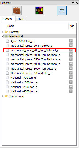
Mechanical Press Library
Generate DB
Check the data and generate the DB. After generating DB switch to ![]() mode to run the simulation.
mode to run the simulation.
Running simulation
Click on the ![]() action label to open the Run Options dialog Use the default Continue Run option to select “Continue from the last step ” option and then select the Simulation mode as Interactive and click on
action label to open the Run Options dialog Use the default Continue Run option to select “Continue from the last step ” option and then select the Simulation mode as Interactive and click on ![]() button to run the simulation.
button to run the simulation.
After simulation complete, switch to ![]() tab.
tab.
Post processor
In Step Browser click on ![]() button to view all steps. Play through the steps to see the deformation.
button to view all steps. Play through the steps to see the deformation.
Point Tracking:
Click on the ![]() and select several points on the workpiece as shown in Fig. 3DL5.74. Click on
and select several points on the workpiece as shown in Fig. 3DL5.74. Click on ![]() and click
and click ![]() for point tracking window.
for point tracking window.
Then click Temperature state variable. This will plot the Temperature vs. Time for all the points that you selected.
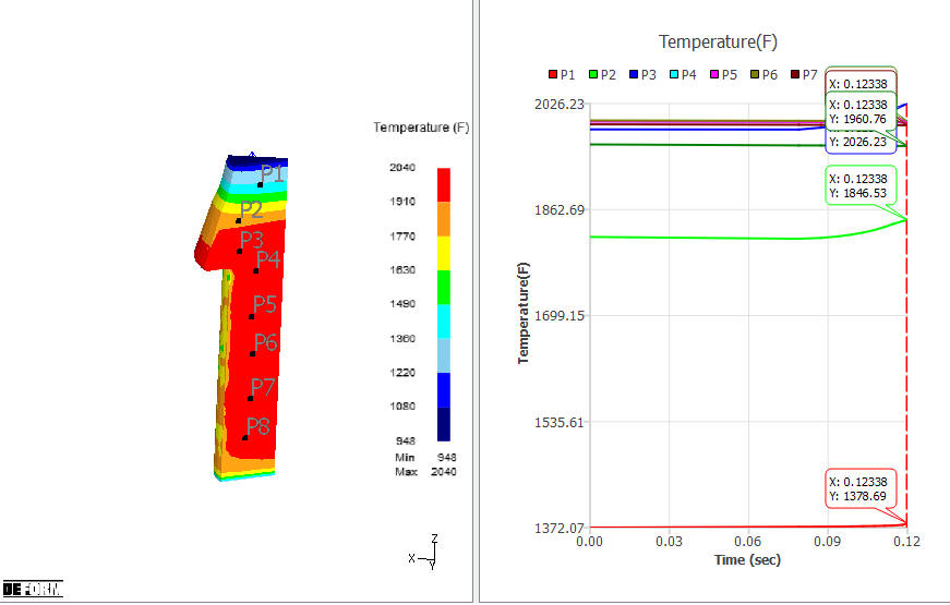
Point Tracking Graph