29.1. Cogging Setup

29.1.1. Cogging Terminology

29.1.2. Die Positioning Method

29.1.3. How to add Cogging operation

29.1.4. Process window

29.1.5. Cogging cycle operation

29.1.6. Pass Table

29.1.7. Material List

29.1.8. Object window

29.1.9. Billet

• Geometry

• Mesh

• Material

• Boundary Conditions

• Property

29.1.10. Top Die

• Geometry

• Mesh

• Material

• Movement controls

• Properties

29.1.11. Manipulators

• Left manipulator1

• Geometry

• Mesh

• Material

29.1.12. Positioning

29.1.13. Scheduled Positioning

29.1.14. Contact (Inter-Object relations)

29.1.15. Simulation preview

29.1.16. Simulation controls

29.1.17. Generate DB

29.1.18. Running Simulation

29.1.19. Post Processing

The cogging operation guides the user to setup the process in simple manner using Passtable, Reheat settings, Primitives and Movement controls. The Pass table helps the user to setup cogging operation in a single action with the movement and rotation of the billet entered, it also accounts for the cooling of the billet between blows and while resting on the bottom die. The pass table helps the user to setup multiple passes easily, by copying settings from one pass to other. The operation can be set using either two dies or four dies as per user requirement.

The cogging wizard provides adaptive reheating option for the user to reheat thebillet when the temperature drops below critical temperature, the billet is reheated and forming operation is continued.

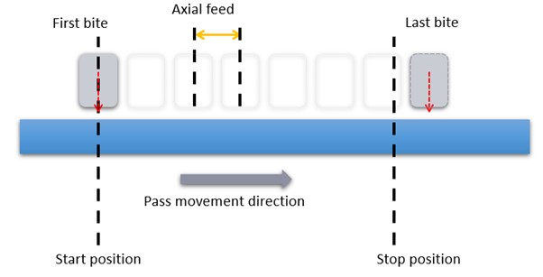
Cogging Terminology

Auto Calculate Bites : By activating this option, system will automatically calculate the no. of bites to be simulated for the given Billet length and axial feed per bite.

Number of Bites : By using this option, user can define required no. of bites for the cogging simulation manually.

Axial Feed per bite: It is the distance that a die set moves per bite in axial direction (Nominal Bite).

E.g.: - if we define axial feed rate as 10 mm, the die set will travel 10 mm down the length of the billet after each bite.

Cross-Section Thickness : Cross-section thickness is the thickness to be maintained on billet in the direction of primary die movement. It is also used as stopping control and also to position dies initially. Depending on the cross-section thickness and number of steps, displacement per step is automatically calculated by system.

E.g.: - if the work piece thickness is 20 mm and we define cross section thickness as 19 mm, simulation is stopped once after achieving the thickness of 19mm on billet in the primary die direction. If any other movement apart from speed is selected, depending on the type of movement the dies are positioned such a way that thickness of 19mm is achieved by the end of deformation operation.

Movement Direction : It specifies the Die movement direction along workpiece axis (+X or -X).

Rotation per Bite (Deg): By using this option user can set the angle for the billet to rotate after each bite.

Rotation per Pass (Deg) : By using this option user can set the angle for the billet to rotate before each pass.

Dwell Time before pass : Using this user can set the time that workpiece rests on the die before the starting of the cogging pass.

Transfer Time Before Pass : Using this user can set the time lapse from the furnace to the cogging pass table before the starting of the cogging pass.

Die Positioning Method

1. 0 -% (Percentage or fraction of billet length between 0 to 1) : Start or stop position is specified as a fraction of the billet length from the respective billet ends, taking cogging direction into consideration.

2. 1 – ref (Reference points): Start or stop position is specified by picking two points on the billet, only the x coordinates are displayed in the table.

3. 2 – dst (Absolute distance from billet ends): Start or stop position is specified by distance from respective billet ends, taking cogging direction into consideration.

4. 3 -ofst (Offset): Start position is specified as a relative distance from previous die position.

Die start position : Die center is the datum point used for initial position for each pass in its movement direction. (See Fig. 29.1.1.).

Die stop position: This option is enabled only when the option ’Auto-calculate bites’ is checked. Pass ends before the die center reaches the given end position.

Die start and Die stop position.

**1.** 0% (Percentage or fraction of billet length between 0 to 1) :
Die start position : Die center is positioned at given distance (specified as a fraction of current billet length) from start of billet in the pass movement direction.(See Fig. 29.1.2.)

Die stop position : Pass ends when die center reaches given distance (specified as a fraction of current billet length) from end of billet in the opposite direction of the pass movement direction.

Default values are zeros, which means the die center is positioned at the start end of billet and stops until it reaches the other end.

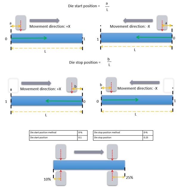
(0-%) Percentage or fraction of billet length die positioning method

2.1 -ref (Reference points) : When this method is selected, picking is enabled and two points on the billet can be picked.

Start point should be picked after clicking on the cell ‘Die start position’ in the first pass. (See Fig. 29.1.3.)

Stop point should be picked after clicking on the cell ‘Die stop position’ in the first pass.

Die center is positioned at the start point and the pass ends when it reaches the stop point. The same two reference points are used for all passes. The reference points are tracked on the deforming workpiece.

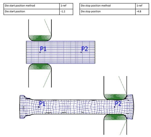
(1-ref) Reference point die positioning method

3.2-dst (Absolute distance method) :
Die start position : Die center is positioned at a given distance from the start of the billet in the pass movement direction. (See Fig. 29.1.4.)
Die stop position : Pass ends when the die center reaches the specified distance from the end of the billet in the opposite direction of the pass movement direction.

Negative values can be used for start and/or end positions.

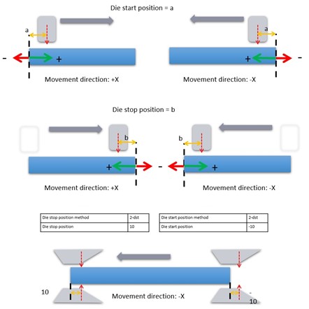
(2-dst) Absolute distance die positioning method

_****4.**3-ofst (Offset method)_ :
**Die start position : Die is moved by the specified distance from its last position. A positive value moves the die in the pass movement direction while a negative value moves it in the opposite direction. (See Fig. 29.1.5.)

Die stop position : Not applicable, this method cannot be used for stopping method as it is not meaningful.

Offset method can be used with a zero value for the first pass if user wants to do manual positioning only. In certain processes, like infeed swaging for instance, dies need to be positioned in a certain specific configuration with reference to the billet. In such cases, the offset position method can be used with a zero value for the first pass. No additional die positioning is done by the system.

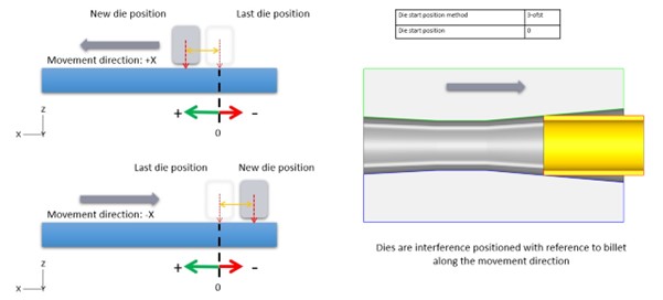
(3-ofst) Offset die positioning method

• Bites to Skip

Number of Bites to skip, this option is applicable for Crank press based movement controls only. Using this option user can set Number of bites to be skipped between each bite in the respective pass of the simulation.

Below Fig. 29.1.6. shows cogging process with two passes, where in first pass we skipped two bites for every bite and in second pass we do not skip any bites.

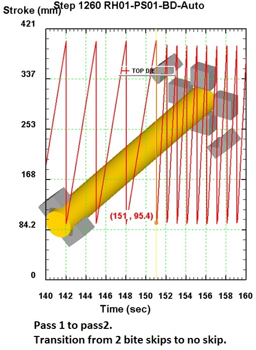
Bite skip

How to add Cogging operation

Cogging operation is accessible from MO Wizard that can be opened from Main GUI. In MO wizard, Cogging Operation can be added from explorer tab by clicking on button next to 3D Cogging. Also, user can add the operation by drag and drop into the Operation Editor as shown in Fig. 29.1.7.

Added Cogging operation in Operation Explorer

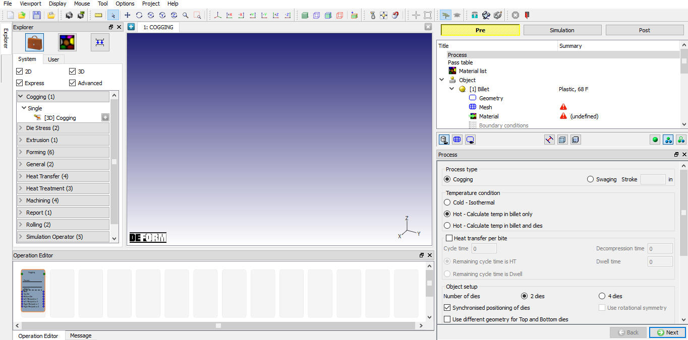
Process window

Below Fig. 29.1.8. shows the options to set the process conditions, these options are explained below.

Process window

Process type

• Cogging : It is a process of increasing length of billet by decreasing the diameter of billet.

The objective of Cogging is modeling of billet conversion process consisting of multiple bites/passes/re-heats in a single operation with automatic stops and restarts between each step of the process.

Cogging wizard is used to generate the master files and the billet, die and manipulator keyword files with necessary information about process, geometry and materials to run a typical cogging simulation.

• Swagging : Modelling of rotary forging processes is known as Swagging.

Temperature Condition

• Cold Isothermal: In this process, we will be able to see only Deformation of Billet.

Note : If we select Cold Isothermal Radio button Heat transfer options would get into greyed out mode.

• Hot - Calculate Temp in Billet Only : In this process, we are able to calculate temp in billet only. As no thermal calculations are carried over on dies and manipulators, no mesh is generated for them. We will able to perform both Heat Transfer and Deformation operations.

• Hot - Calculate Temp in Billet and Dies : In this process, we are able to calculate temp in billet, dies and manipulators. All objects should be meshed as we need to perform thermal calculations on billet, dies and manipulators. We will able to perform both Heat Transfer and Deformation operations.

Heat Transfer Per Bite

It is nothing but, how much time we want to transfer Heat per a particular bite.

• Cycle Time : Cycle time is the total time lapse between two successive bites. In a typical cogging operation it is the summation of, Bite Deformation + Bite Decompression time + Bite Dwell + Bite heat.

• Decompression Time: It is the time lapse before dwelling operation is started and after deformation operation is completed. During this time both top dies and bottom dies will be in contact with the Billet.

• Dwell Time: It is the time lapse between decompression time and the commence of next bite. During this operation only bottom die will be in contact with die.

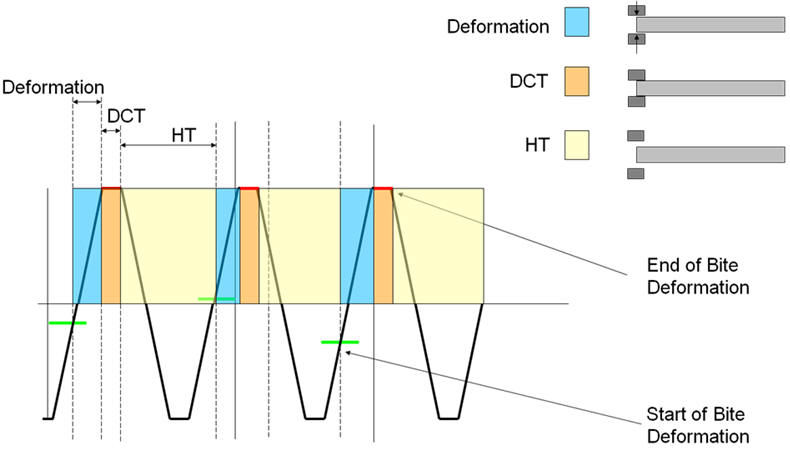
• Remaining Cycle Time as HT: In a case where the forging stroke is reached before the completion of cycle time, the remaining time of cycle is considered as Heat Transfer operation during which both the dies will be in contact. (See Fig. 29.1.9.)

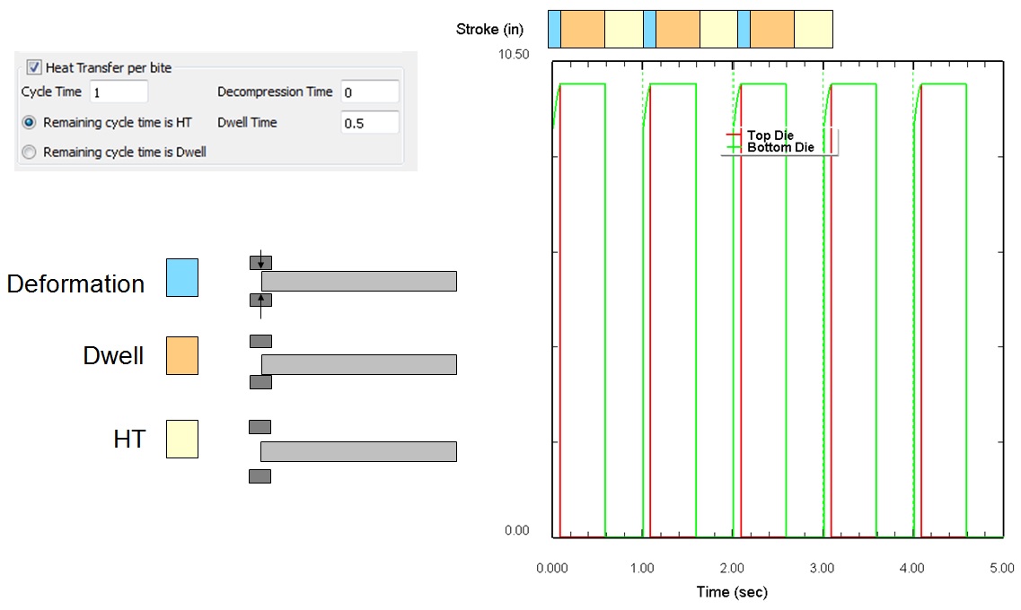
Remaining cycle Time as HT

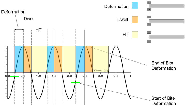
• Remaining Cycle Time as Dwell : In a case where the forging stroke is reached before the completion of cycle time, the remaining time of cycle is considered as Dwell during which the top die moves away from the billet. (See Fig. 29.1.10.)

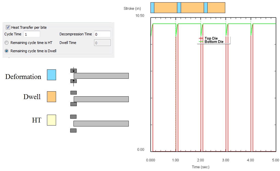
Remaining Cycle time as Dwell

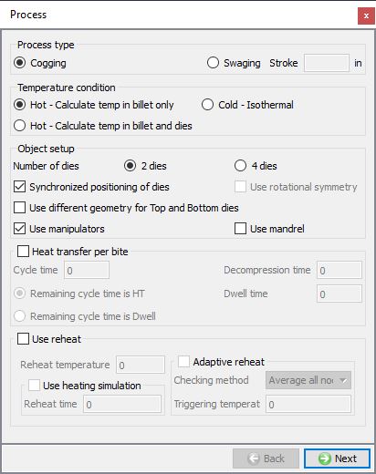
Object Setup

• Number of Dies : Cogging process is carried out either b using 4 dies or 2dies depending on the cross-section and amount of deformation. User can select either 4 Dies or 2 Dies based on the process to be simulated.

• Use different geometry for Top and Bottom dies : In cogging process if the geometries in a die set are different then by checking this checkbox we will be able to define different types of geometries for Top die and Bottom die.

• Use Manipulators : If manipulators are used then user can turn on this check box to activate Manipulator definition and its settings.

• Use Mandrel : By checking this checkbox user will be able to use Mandrel for the setup where hollow workpieces are processed. It is used especially for the swagging setup.

• Use rotational symmetry : By checking this checkbox, user will be able to define symmetry on the workpiece, see Fig. 29.1.8. Using symmetry the simulation time can be reduced.

Use Reheat

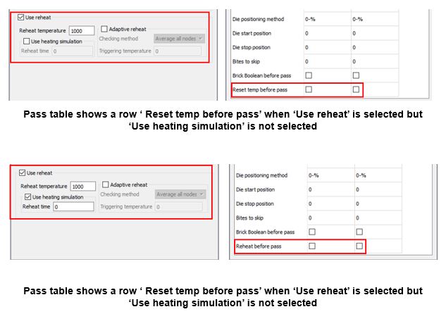
“Use Reheat” checkbox can be turned on to reheat the billet at the end of pass. The billet can be reheated adaptively based on the specified “Triggering Temperature” or can be scheduled between passes by turning on the “Reheat” checkbox in the pass table. Reheating billet can be simulated for “Reheat time” period by turning on “Use heating simulation” checkbox or can be initialized to “Reheat Temperature” by turning off “Use heating simulation” checkbox. (See Fig. 29.1.8.)

• Reheat Temperature : It is the temperature to which the billet has to be reheated for the forming process to be started.

Use heating simulation

When selected, a heating simulation is added with Reheat temperature as environment temperature for period of “Reheat time” before the selected pass. If “Use Reheat” is checked and “Use heating simulation” is unchecked, then only nodal temperature is initialized to Reheat temperature before the selected pass.

Use Adaptive heat

Cogging is very lengthy process during which the billet temperature will drop down below forging temperature at certain point, by checking this adaptive heat checkbox, automatically system reheats the billet to forging temperature specified and continues the cogging process. Adaptive Reheat will takes place between passes only. (See Fig. 29.1.8.)

• Checking Criteria

• All Nodes : User can select this option when the reheating process is to be triggered when temperature at all nodes in the billet goes below the assigned triggering temperature.

• Average of all Nodes : By selecting this radio button, the reheating process is triggered when average temperature of all nodes in the billet goes below the assigned triggering temperature.

• Any Node : By selecting this radio button, the reheating process is triggered when any one node temperature goes below the triggering temperature.

• Average Surface Nodes : By selecting this radio button, the reheating process is triggered when average surface nodes temperature goes below the assigned triggering temperature.

• Triggering Temperature : It is the temperature at which the reheating of the billet should be triggered.

Pass table

New row has been added at the end where user can schedule Reheat for individual passes using check box (See Fig. 29.1.11.). This row will be hidden when no Reheat options are selected or if Adaptive heating has been selected.

Pass table options with Use Reheat option

Cogging cycle operation

Cogging process involves several operations. A typical sequence of operations involved in cogging process is explained here. The below Fig. 29.1.12. shows the operations performed on billet before cogging process is started.

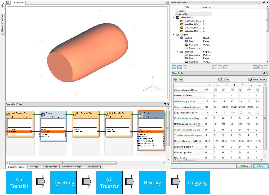
Multiple Operation setup

Following are the operations involved in a typical cogging pass that can be setup as sequence in DEFORM using cogging wizard process parameters and pass table window.(See Fig. 29.1.13.)

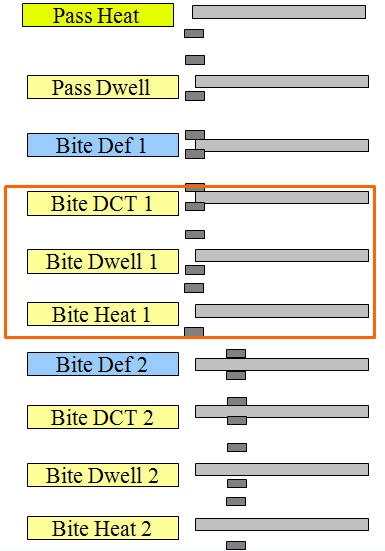
Operation involved in a typical pass

Based on the process requirement, user can control the operations to be performed and its settings. Below Fig. 29.1.14. and Fig. 29.1.15. shows difference in operation cycle when decompression time is not used and used.

Operation cycle without Decompression Time

Operation cycle with Decompression Time

Pass Table

Below Fig. 29.1.16. shows the Pass Table. In this table we will define the information of entire pass for the cogging setup. Various options available in pass table are explained in Cogging Terminology. Pass information is copied from previous pass whenever a new pass is added and necessary information can be edited based on the process requirement. Please refer 29.1.1. cogging Terminology.

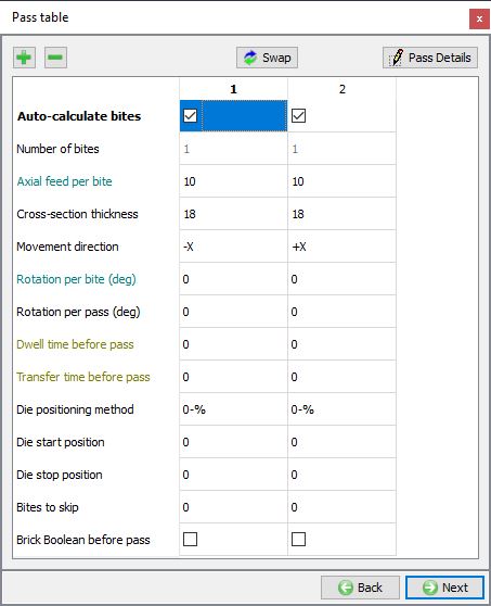
Pass Table Window

Button: This button is used to increment pass by one.

Button: This button is used to delete the existing pass.

New passes can now be inserted anywhere in the pass table, not just at the end. (see Fig. 29.1.17.)

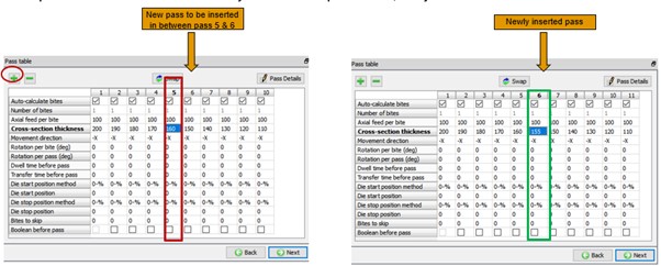
Adding new pass between 5 and 6

: If we click on swap button, the pass parameters are arranged horizontally for display.(see Fig. 29.1.18.)

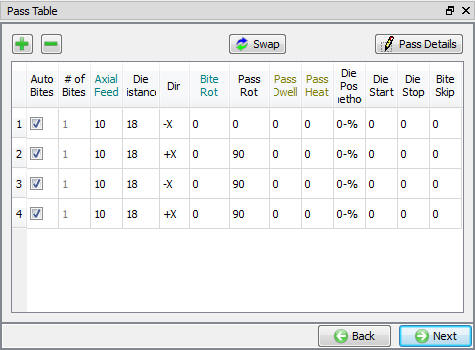
Showing Pass table information in Horizontal Direction

:User can use this option to enter advanced pass information applicable to all passes, see Fig. 29.1.19.

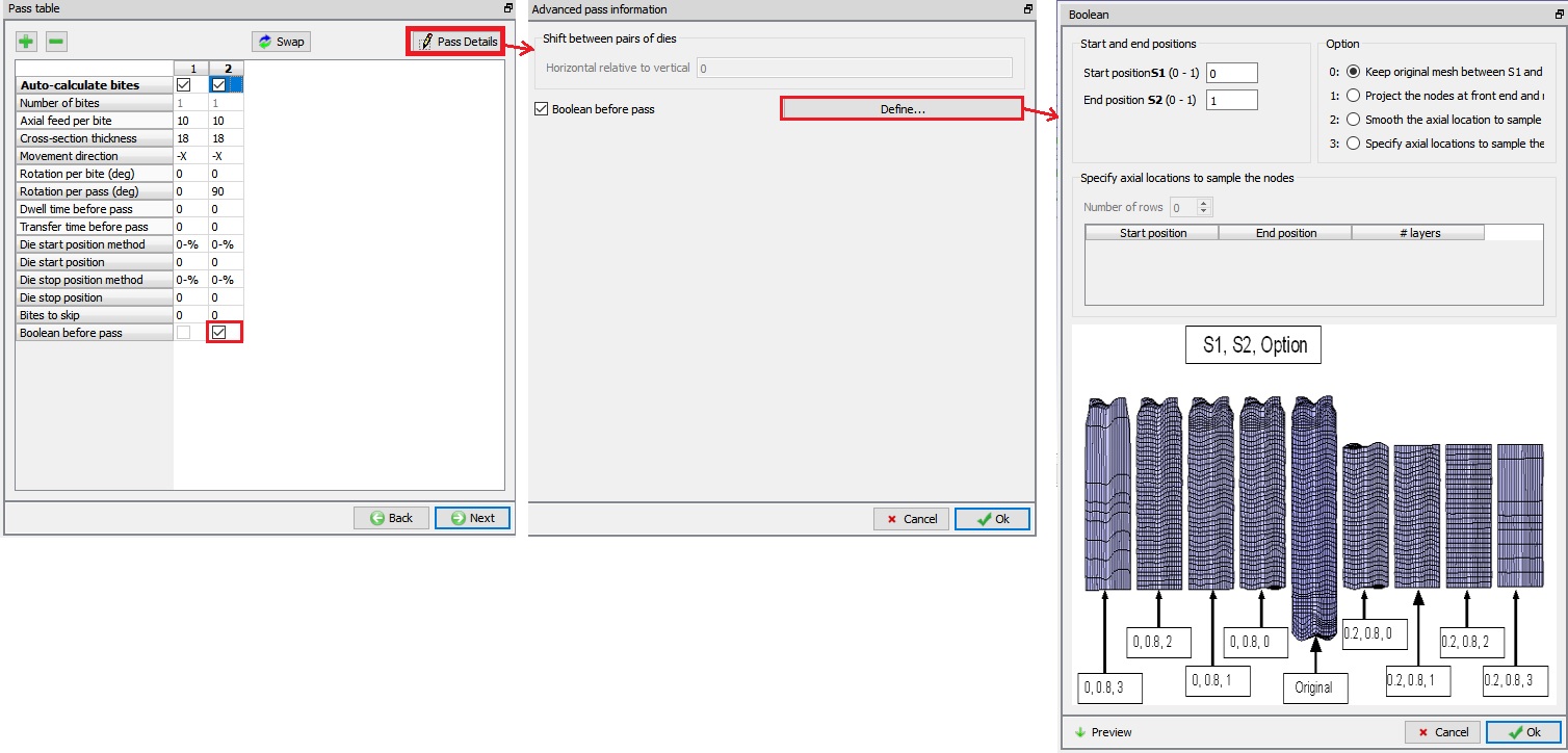
Advanced Pass Information window

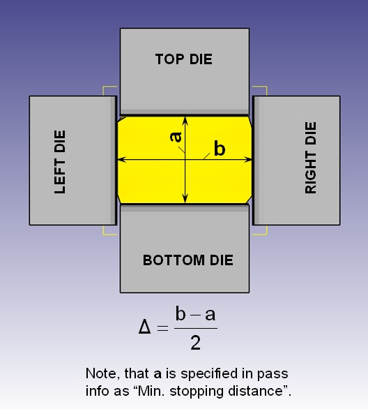
Shift between pairs of dies:

This option is applicable only when 4 dies are used for cogging and the amount of the deformation, i.e. forging stroke, is different for horizontal set of dies and vertical set of dies.

As show in Fig. 29.1.20., Shift distance Δ = (b-a)/2

Where

Δ is the Shift between pairs of dies

a is the Min. Stopping distance between Top and Bottom dies

b is the Min. Stopping distance required between Left and Right dies

Shift between the pairs of dies at the end of the bite

If we use the positive value for shift between pairs of dies (Δ) then only the side dies (left and right dies) will shift away from the workpiece by this absolute value at the beginning of the every bite.
So that distance between horizontal left and right dies at the end of the bite is more, twice the Δ value than the distance between vertical Top and bottom dies. This means the workpiece deformation along vertical direction is twice the Δ than the horizontal direction.
But if we use negative value for shift between pairs of dies (Δ), then Top and Bottom dies will shift away from the workpiece by this absolute value.

Boolean before Pass: Option to trim the billet between passes as it elongates beyond desired length. (see Fig. 29.1.21.) For more information related to Brick boolean before pass option refer 43.1. Shape Rolling Manual : Boolean between passes section

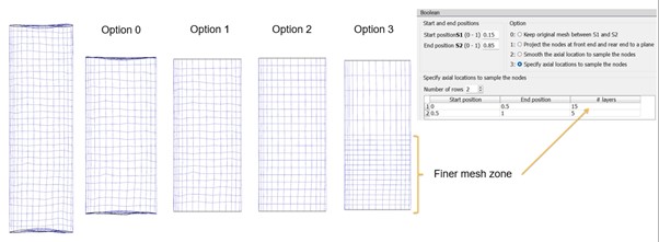
Brick boolean with all options for Start position 0.15 and End position 0.85

From v14, Boolean operation between the passes can be added even for the workpiece with Tet mesh.(See Fig. 29.1.22.).

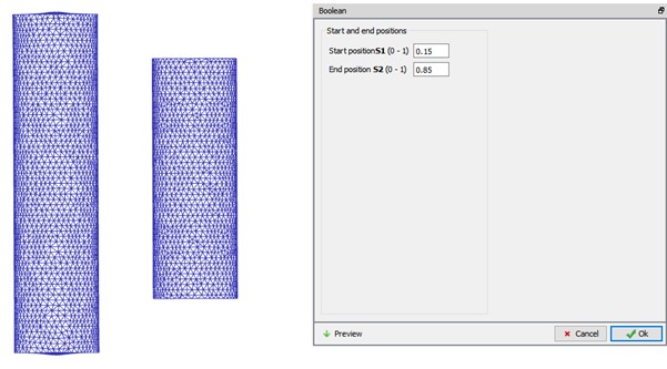
Tet boolean option with Start position 0.15 and End position 0.85

Material List

In order for a simulation to achieve a high level of accuracy, it is important to have an understanding of the material properties required to specify a material used in DEFORM.
When setting up a simulation, material properties have to be specified for the objects. In MO Cogging operation, all the materials required for the operation can be loaded at a time and the required material can be selected later as the problem is setup. User can add material by selecting load material data from library as shown in Fig. 29.1.23. User can select required material from the categories and then click on button as shown in Fig. 29.1.24.

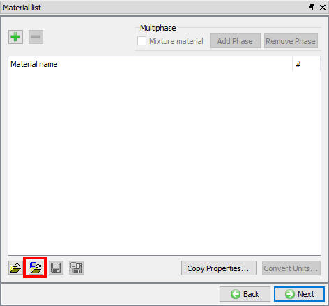
Material list window

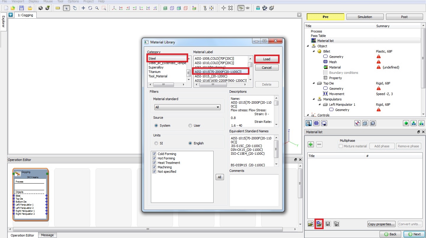
Import material from library window

(or)

Another way of adding material is click on the material icon of the explorer tab, a list of materials from library that are divided into different categories will appear as shown in Fig. 29.1.25. Select required material then click on button. Also, user can add required material by drag and drop into the material window.

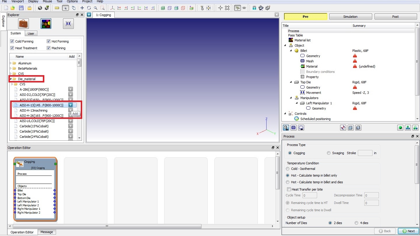
Adding Material from Explorer tab

(or)

In material list window, by clicking on button, new material can be added. After a dding material click and select respective tab to define required data for the simulation as shown in Fig. 29.1.26.

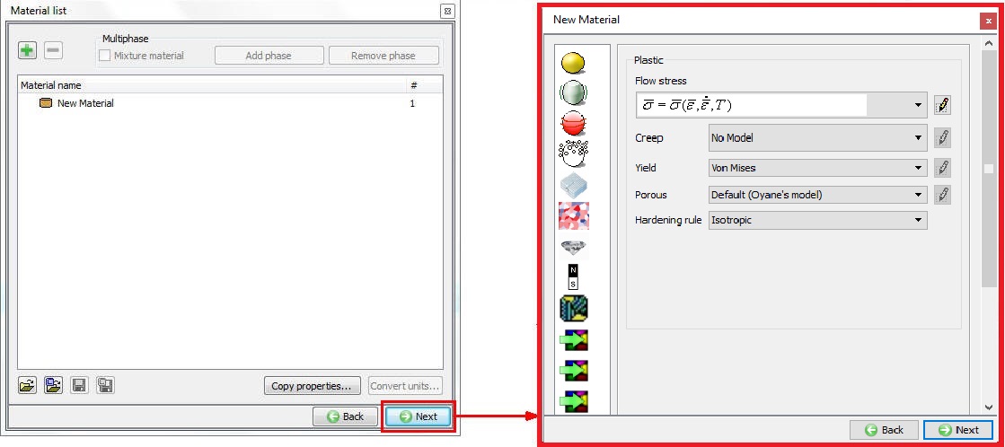
Add material from Material List window

Import Material data from a file : It imports the material from a .Key or .DB file.

Load Material data from Library :It imports material from Library.

Save the Material data to a file : It saves the material to a file.

Save the Material data to Library : User can save material to the library using this option and can be loaded back as required in future for other simulations.

Mixture material

“Mixture” materials (MSTMTR) are used when a phase transformation is to be modeled in the simulation. The transforming material is modeled as a “mixture” of its constituent phases. For example, carbon steel might be modeled as a mixture of Austenite, Pearlite, Bainite, and Martensite. If a mixture material is defined, transformation rules should be defined which govern the transformation of one phase into another.(See Fig. 29.1.27.)

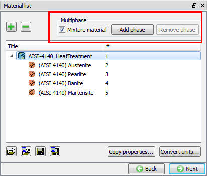
Adding Mixture material

Copy Properties

It is used to copy the regular material properties like plastic, elastic, thermal etc. from one material to other while creating/defining the material data as shown in Fig. 29.1.28. In this dialog, source and destination for copying the properties and properties to be copied must be selected.

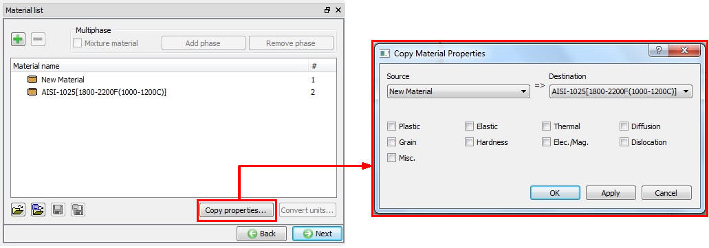
Copy material properties window

Convert Units

It is used to convert the unit system of current selected material from material list from SI to English or English to SI or user can use any other multiplication factor as shown in Fig. 29.1.29. Selecting the button will display the respective multiplication factors for converting from and , then selecting the Convert button will convert and close the conversion window. This conversion table can be saved using save button and can also be edited by using wordpad/notepad and loaded back UNITCONV.DAT file using load button.

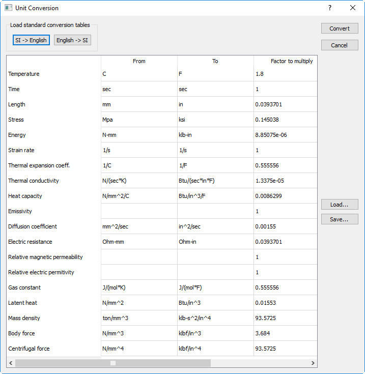
Unit Conversion window

Object window

Below Fig. 29.1.30. shows the object window information.

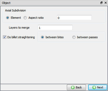
Object window

Axial Sub Division: Element: Absolute size of the element is specified in the field, if the element size increases beyond the specified value then axial sub-division takes place to maintain the element size.

Aspect ratio : Aspect ratio: It is the ratio of the minimum edge length to maximum edge length of an element. In cogging, most of the times the billet expands in axial (X) direction as the cross-section is reduced (Z or Y), hence the ratio normally would be element length in X direction to minimum of element length in Y or Z direction.
When aspect ratio exceeds the value specified, axial sub-division takes place to maintain the ratio. (See Fig. 29.1.31.)

Axial subdivided workpiece mesh while simulation in progress

Layers to merge: Cogging is an ingot conversion process in which the length of the billet is large and the deformation zone at an instant is less compared to length of the billet. Hence, to reduce the simulation time user can indicate the layers that can be treated as one so that same result is reflected across the specified number of layers.

Do billet Straightening

• Between Bites : During cogging process there is tendency that billet might bend and by selecting this radio button billet can be straightened between Bites.

• Between Passes: By selecting this radio button billet can be straightened between passes.

Billet

In this window user can define required temperature for the object and select type of the object as shown in Fig. 29.1.32. For billet by default the object type selected is Plastic. User can also import object from other DB’s or Keyfile’s using button and browsing respective file.

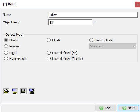
Assigning temperature for billet

Geometry

Geometry window is used to define the geometry of an object as shown in Fig. 29.1.33. Only define primitive field will be in active mode rest other options will be in greyed out mode when no geometry is defined. Once after creating geometry all the options will be activated.

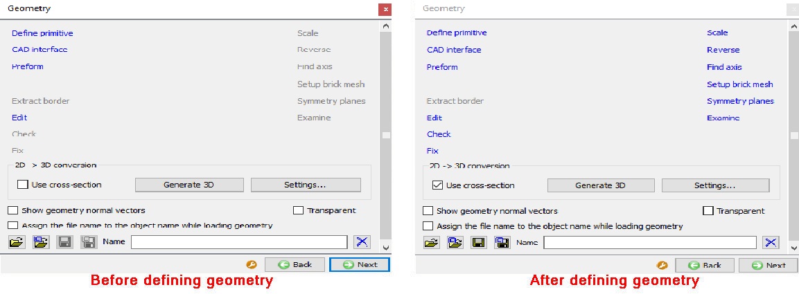
Geometry Window

Define Primitive

We have three different types of Geometry primitives for billet, Ring, Octagon and Rectangle as shown in Fig. 29.1.34.

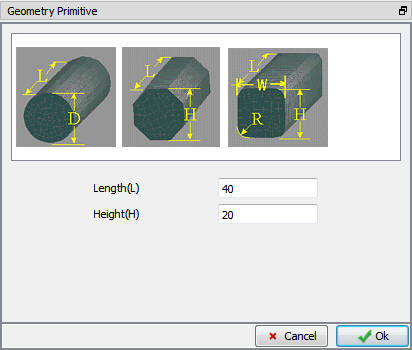
Geometry primitive window

For more information about geometry options, please refer 12.3. 3D Geometry Data Definition

Mesh

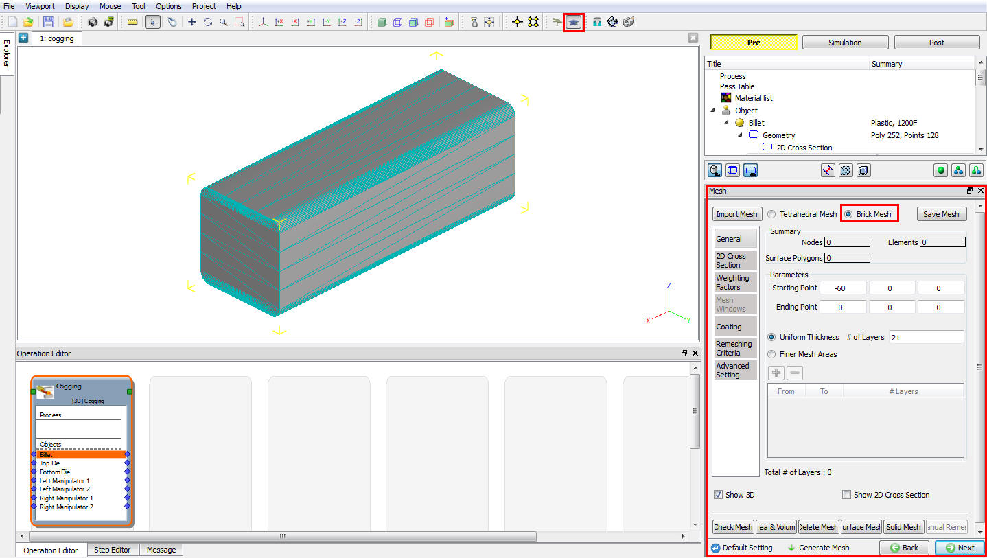
Brick mesh

The below Fig. 29.1.35. shows the mesh generation options for Brick Mesh in guided mode.

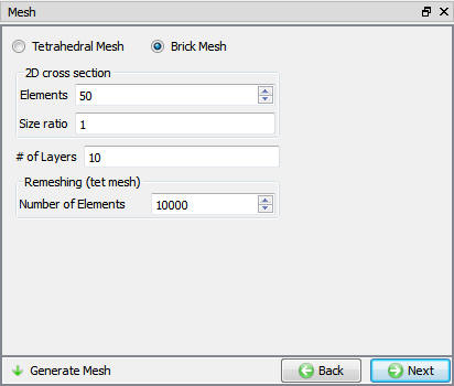
Brick Mesh options in Guided mode

2D cross section

• Elements : The number of mesh elements represents the approximate number of elements that will be generated on a 2D cross-section of an Object.

• Size Ratio : Size ratio is the ratio of maximum element size to minimum element size on 2D cross-section.

• No. of Layers : It is used to control the thickness of mesh layers in axial direction. User can define the required number of layers for the mesh generation. As number of layers is increased, mesh will be denser and the thickness of the element decreases in axial direction. similarly, if number of layers is decreased then element thickness in axial direction will be increased and will see less number of layers.

• Remeshing (Tet mesh) : If there is a huge deformation and brick mesh fails to go for remeshing, then system will opt to tetrahedral mesh automatically and generates mesh based on the settings defined.

• Number of Elements : The number of mesh elements represents the approximate number of elements that will be generated on an Object. The defined number of elements will be taken, when it hits the tetrahedral remeshing.

• Generate Mesh : The mesh can be generated by clicking .

Tetrahedral Mesh

The below Fig. 29.1.36. shows the mesh generation options for Tetrahedral Mesh in guided mode.

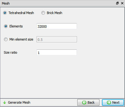
Tet mesh options in Guided mode

• Elements : The number of mesh elements represents the approximate number of elements that will be generated that will be generated on an Object.

• Min Element Size : It is the minimum size of the element, while generating mesh it will create the element with respect to the defined minimum element size. Element size will not exceed the defined value.

• Size ratio : Size ratio is the ratio of maximum element size to minimum element size on an object.

• Generate Mesh : The mesh can be generated by clicking .

In order to control the mesh parameters like size, shape, density, type of elements, etc…, user has to switch to expert mode for more advanced mesh options. Below Fig. 29.1.37. shows the mesh options available from Expert mode.

Expert mode Mesh generation window

For more information about expert mode mesh generation options please refer, 13.2. 3D Tet Mesh Generation and 13.3. 3D Brick Mesh Generation

Material

Below Fig. 29.1.38. shows the material window. User can assign required material from the list or can import from file or library. User can also add new material. For more information on how to assign material, Please refer chapter 10. Material Data

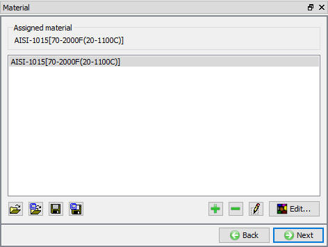
Material window

Once after adding material click on button, material window will open as shown in Fig. 29.1.39.

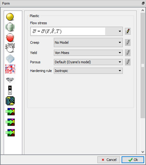
Edit material window

The properties required are dependent on the physical effects being simulated in DEFORM. The material properties that the user is required to specify is a function of the material types that the user is utilizing in the simulation. For more information, Please refer Material in Forming 3D setup.

Boundary Conditions

In Boundary conditions window, user can assign various boundary constraints for an object. Boundary conditions specify how the boundary of an object interacts with other objects and with the environment. The most commonly used boundary conditions in cogging are heat exchange with the environment for simulations involving heat transfer, prescribed velocity for enforcing symmetry. Fig. 29.1.40. shows various BCC that can be assigned to an object.

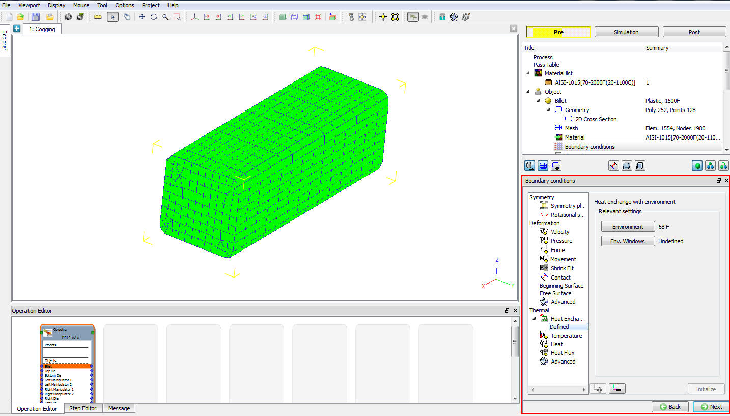
Boundary Conditions window

The BCC’s are categorized as Deformation,Thermal, Diffusion and Heating. For more information about these BCC’s please refer 14. Boundary Conditions.

Property

Miscellaneous object parameters, which affect either thermo-mechanical behavior of the object or numerical solution behavior are specified in the Object-Properties window. (See Fig. 29.1.41.). For more information on these options, Please refer 19. Object properties.

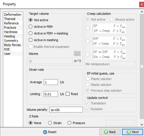
Object property window

Top Die

In this window, user can define required temperature for the object and select type of the object as shown in Fig. 29.1.42. For Top Die by default the object type selected is Rigid and user can also import object from other DB’s or Keyfile’s using button and browsing respective file.

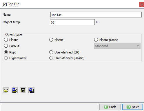
Top Die window

Geometry

Geometry window is used to create the geometry of an object as shown in Fig. 29.1.43. Only define primitive field will be in active mode rest other options will be in greyed out mode when no geometry is created. Once after creating geometry all the options will be active.

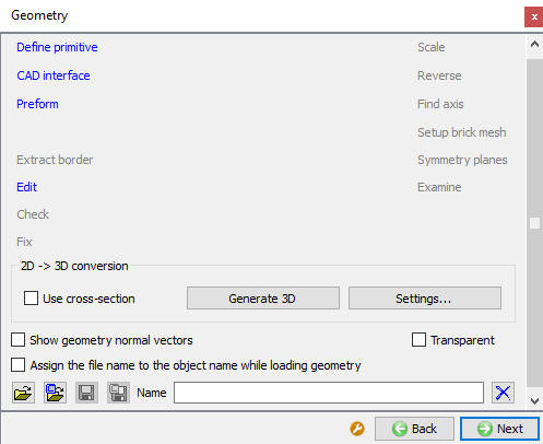
Geometry window

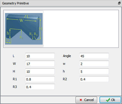
Define Primitive

Below Fig. 29.1.44. shows the Geometry primitive of Die.

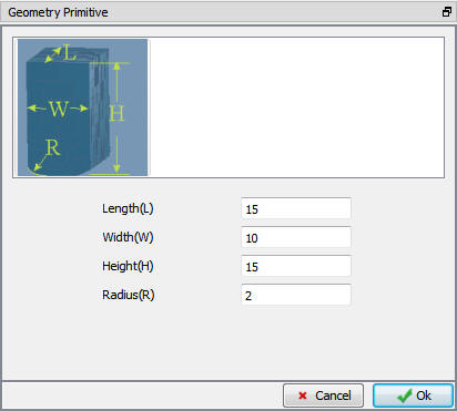
Top Die Geometry Primitive window

For more information about geometry options please refer 12. 3. 3D Geometry Data Defining

Mesh

Mesh generation options for Dies are similar to that of the billet, for more information on Mesh generation please refer 3.3. 3D Brick Mesh Generation

Material

Assigning material to dies is similar to that of billet. User can assign required material from the list or can import from file or library. User can also add new material. For more information on how to assign material, Please refer chapter 10. Material Data

The material properties that the user is required to specify is a function of the material types that the user is utilizing in the simulation. This section describes the material data that may be specified for a DEFORM simulation. For more information, Please refer Material in Forming 3D setup.

Movement controls

Depending on the process requirement and equipment used user can define movement control settings for dies. For a quick Cogging setup, Speed and Mechanical press movement controls will be used as shown in Fig. 29.1.45. If user want to define other movement controls than these, then advanced radio button can be used by clicking button, these options can also be accessed by switching to Expert mode as shown in Fig. 29.1.46. For more information about these movement controls, please refer 10. Movement Controls Definition.

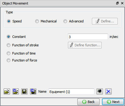
Guided Mode Movement controls window

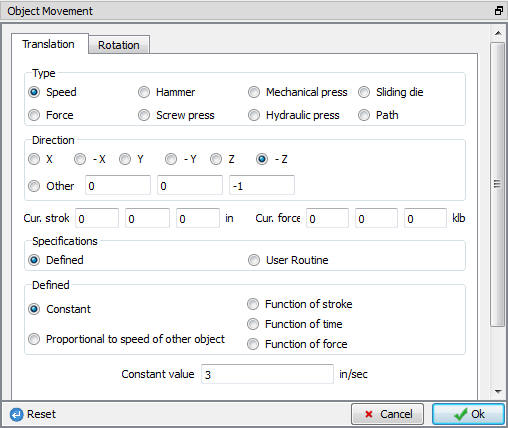
Expert mode movement controls window

Object Property

Die reference Points:
By checking the “Define reference point ” check box, user can specify the reference point for the Cross-section thickness. If the check box is not turned on, then the system places a virtual bounding box over the dies and uses it to measure the Cross-section thickness as illustrated below (See Fig. 29.1.47. and Fig. 29.1.48.).

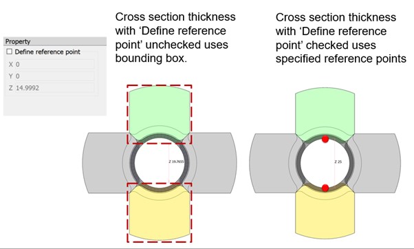
Defining reference point (Right) and using system default reference point option (Left)

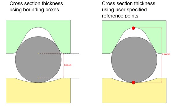
Defining Reference point for Asymmetric dies

Manipulators

Start position wrt billet ends : Manipulators will be positioned axially at a distanced specified here from the billet end face.

Use master manipulators : By checking this checkbox, user will be able to select the required (left or right) manipulators as priority to hold the billet during the simulation.
If user selects Left manipulators as master manipulator then whenever Dies reaches assigned hand over distance, only Left manipulator will hold the billet. Similarly if Right manipulator is selected as master manipulator then whenever Dies reaches assigned hand over distances, only Right manipulator will hold the billet

Use spring loaded manipulators: Manipulators can be defined as spring loaded or rigid. Spring loaded manipulators can be defined by turning on this checkbox. The parameters required to control the spring load manipulators are set here (spring stiffness, preload and maximum spring displacement allowed). (See Fig. 29.1.49.)

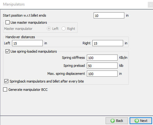
Manipulators window

Left manipulator1

In this window, user can define required temperature for the object and select type of the object as shown in Fig. 29.1.50. For manipulator by default the object type selected is Rigid and user can also import object from other DB’s or Keyfile’s using button and browsing respective file.

Left Manipulator1 window

Geometry

Geometry window is used to create the geometry of an object as shown in Fig. 29.1.51. Only define primitive field will be in active mode and rest other options will be in greyed out mode. Once after creating geometry all the options would get active.

Geometry Window

Define primitive

Below Fig. 29.1.52. shows the Geometry primitive of Manipulator available in Cogging wizard.

Manipulator Geometry primitive window

Mesh

Mesh generation options for Dies are similar to that of the billet.

Material

Assigning material to dies is similar to that of billet. User can assign required material from the list or can import from file or library. User can also add new material.

Positioning

Below Fig. 29.1.53. shows the positioning window.

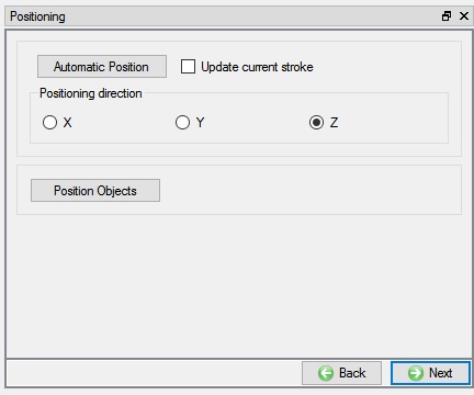
Controls window

Positioning of dies and manipulators is controlled automatically by system in cogging wizard and user requires these positioning options rarely, whenever dies are imported externally. Positioning top die would be sufficient, as the template automatically replicates the position for other dies. In a fresh setup only Top die is visible for positioning and even though other dies are positioned manually while editing a setup they are not stored, only the top die position is stored and reflected on the other dies. For more information on these positioning options please refer to below sections.

• Automatic Positioning

By clicking on this button, system automatically Positions the Objects with respect to the top die movement direction, this option works best for simple setup with three objects work piece, top die and bottom die.

• Positioning Objects

By clicking on this button, user can position the objects in required directions. Various types of Positioning Options are available such as Drag, Offset, Interference, Flip and Rotational as shown in Fig. 29.1.54. For more information about these options, please refer 16.Object Positioning.

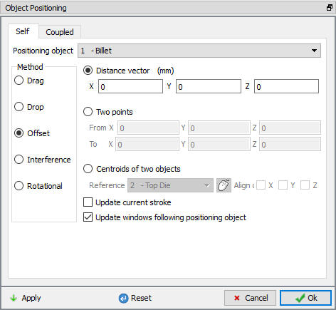
Object positioning window

Scheduled Positioning

Schedule positioning allows the user to define the positioning for objects in MO setup for successive operations for which DB is not generated so that the objects are positioned before generation of DB while running simulation in batch mode. This option is also rarely used in cogging process.

Contact

The purpose of inter-object relations is to define how the different objects in a simulation interact with each other. The relations table shows the current inter object relations that have been defined as shown in Fig. 29.1.44. All objects which may come in contact with each other through the course of the simulation must have a contact relation defined. This includes an object having a relationship to itself, if self-contact occurs as in case of lap. It is very important to define these relationships correctly for a simulation to model a forming process accurately.

System : By selecting this radio button, system assigns default inter-object relationships. Also user can add the lubricants if necessary by selecting Add New from pull down menu and clicking on “Edit” button or user can load the required lubricants from the library for the simulation.

By default in Cogging operation User option is selected, user** would like to define his own relations then user radio button should be selected. User can add relationships by clicking on Add button as shown in Fig. 29.1.55.

Frictional and Heat Transfer Coefficients can be applied even from simulation controls window,

For more information please refer, Inter-Object Relations in Forming 3D setup.

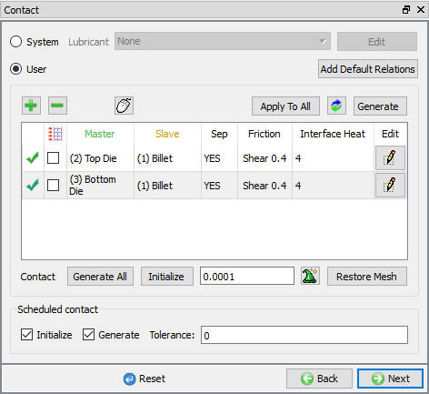
Inter-Object definition window

Simulation preview

Simulation Preview provides an overview of the operations like deformation, dwelling, reheat..etc. to be executed based on the process definition and pass table as animation. It also gives preview of the setup at each operation. In Simulation preview window, by clicking the button animation would be played (See Fig. 29.1.56.).

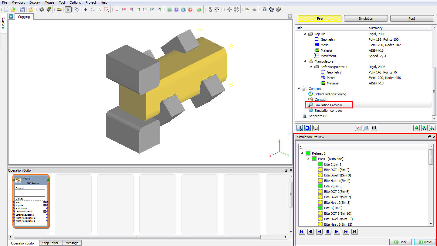
Simulation preview window

Simulation controls

The DEFORM system solves time dependent non-linear problems by generating a series of FEM solutions at discrete time increments. At each time increment, the velocities, temperatures, and other key variables of each node in the finite element mesh are determined based on boundary conditions, thermo mechanical properties of the work
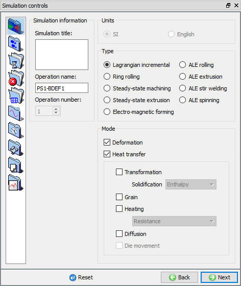
piece materials and possibly solutions at previous steps. Other state variables are derived from these key values, and updated for each time increment. The length of this time step, and number of steps simulated, are determined based on the information specified in the step controls menu. Fig. 29.1.57. Shows simulation control options in Guided mode of cogging operation, the basic options required for forming operation are provided here while Expert mode provides more detailed options.

In guided mode user can define simulation controls for deformation operation and heat transfer operations independently. System will generate .MST file accordingly with the information and apply simulation controls respectively for all the operations to be executed. Frictional and Heat Transfer Coefficients can also be defined here.

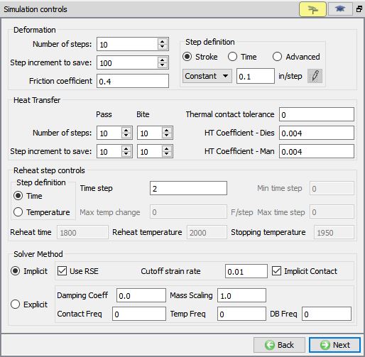
Guided mode Simulation controls window

Deformation

Number of simulation steps (NSTEP)

The number of simulation steps parameter defines the number of steps to run from the starting step number/previous operation. The simulation will stop after this number of simulation steps have run, unless stopping control is triggered to stop the simulation or if the simulation runs into a problem. This setting can be set independently for deformation and Heat transfer operations.

Step increment to save

The step increment (STPINC) to save in the database controls the number of steps that the system will save in the database. When a simulation runs, every step must be computed, but does not necessarily need to be saved in the database. Storing more steps will preserve more information about the process, consequently it will require more storage space. Since Cogging operation is a lengthy process, user should be careful in defining this value so that the .DB file size can be controlled. This setting can be set independently for deformation and Heat Transfer operations.

Friction Coefficient

The coefficient of friction between Dies and billet and Manipulators and billet is set using this option.

Step definition (DSMAX/DTMAX)

Solution step size can be controlled by time step or by displacement of the primary die. If stroke per step is specified, the primary die will move the specified amount in each time step. The total movement of the primary die will be the displacement per step multiplied by the total number of steps. If time per step is specified, the time interval per step will be used. The die displacement per step will be the time step times the die velocity. By default in Cogging operation Top Die is defined as primary die.

The definition of step increment control have been enhanced to include both the time and stroke dependent step functions, these options are available under Expert mode. This means, step size (both time per step and stroke per step) can now be defined as a function of time or stroke. This functionality enables finer resolution of saved model information, where it is desired. (typically towards the end of the stroke, where steep changes of die load can take place)

Heat transfer

HT Coefficient Dies

Heat Transfer Co-efficient between dies and billet is specified here which is applicable to all operations.

HT Coefficient Manipulators

Heat Transfer Co-efficient between manipulators and billet is specified here which is applicable to all operations.

---

Reheat step controls:
Reheat operation simulation steps will be controlled based on the Reheat step definition. We can define either Time or Temperature based Reheat step controls.

For Time based step definition, we need to enter the time for each step.

For Temperature based step definition, we need to enter “Initial time step”, “Max temp change”, Min time step and Max time step” values.

Defined parameters of “Reheat temperature”, “Reheat time” and “Stopping temp” values under Process page will be displayed in respective field.

Solver method

User has an option to select whether implicit solver to be used or explicit solver.

Implicit:

Use RSE: RSE can be activated by turning on this checkbox. For more information on RSE please refer RSE[MO] under 16.Object properties.

Limiting Strain Rate : The limiting strain rate (LMTSTR) defines a limiting value of effective strain rate below which a plastic or porous material is considered rigid and behaves as Newtonian fluid like material.

Implicit Contact : Implicit contact method between objects can be activated by turning on this check box.

Simulation controls in Expert Mode

Fig. 29.1.58. shows the Simulation Controls in Expert mode. For more information and description about options in Simulation controls, Please refer 9. Simulation Controls.

Expert mode Simulation controls

Generate DB

Check Data

It checks the Data. If Data is correct we can generate DB. But while checking Data if it gives any errors or warnings then it should be corrected before generating Database. Errors will not allow the database to be generated while warnings will allow the DB to be generated.

Generate Database

By clicking on this button, it will generate the Database of the setup to start the simulation.(See Fig. 29.1.59.)

Append Key file

Any information that is not defined in the wizard but still applicable to the process can be loaded as .key file. This option is also useful in the cases where only few values needs to be changed then those values can be defined as .key file and only .key file can be changed and simulation can be resubmitted.

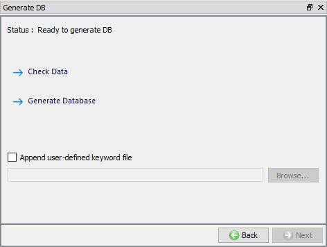
Generate DB window

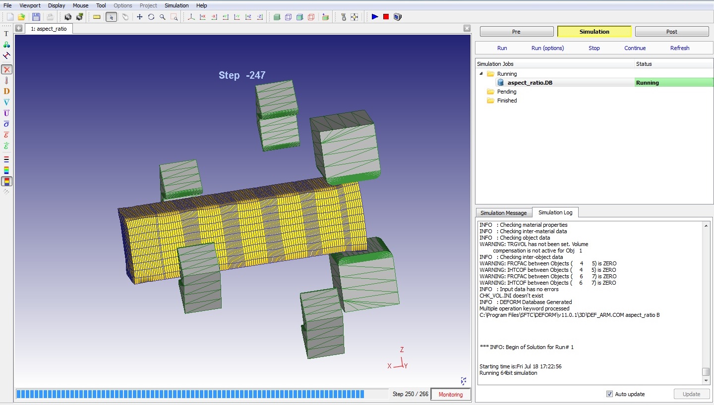
Running Simulation

Once the database has been generated, switch to the Simulation mode by clicking on button above the operation tree. Start the simulation by clicking the action label and selecting run from last negative step option in Run simulation pop-up window.

Monitor the progress of the simulation by looking at the Simulation graphics window, Simulation Message and Simulation Log tabs, making sure that the option is checked (See Fig. 29.1.60.) so that message file and log files are refreshed automatically for monitoring the simulation progress. Simulation graphics tool bar options can be used to plot basic state variables such as temperature, strain and contact for objects while simulating the problem.

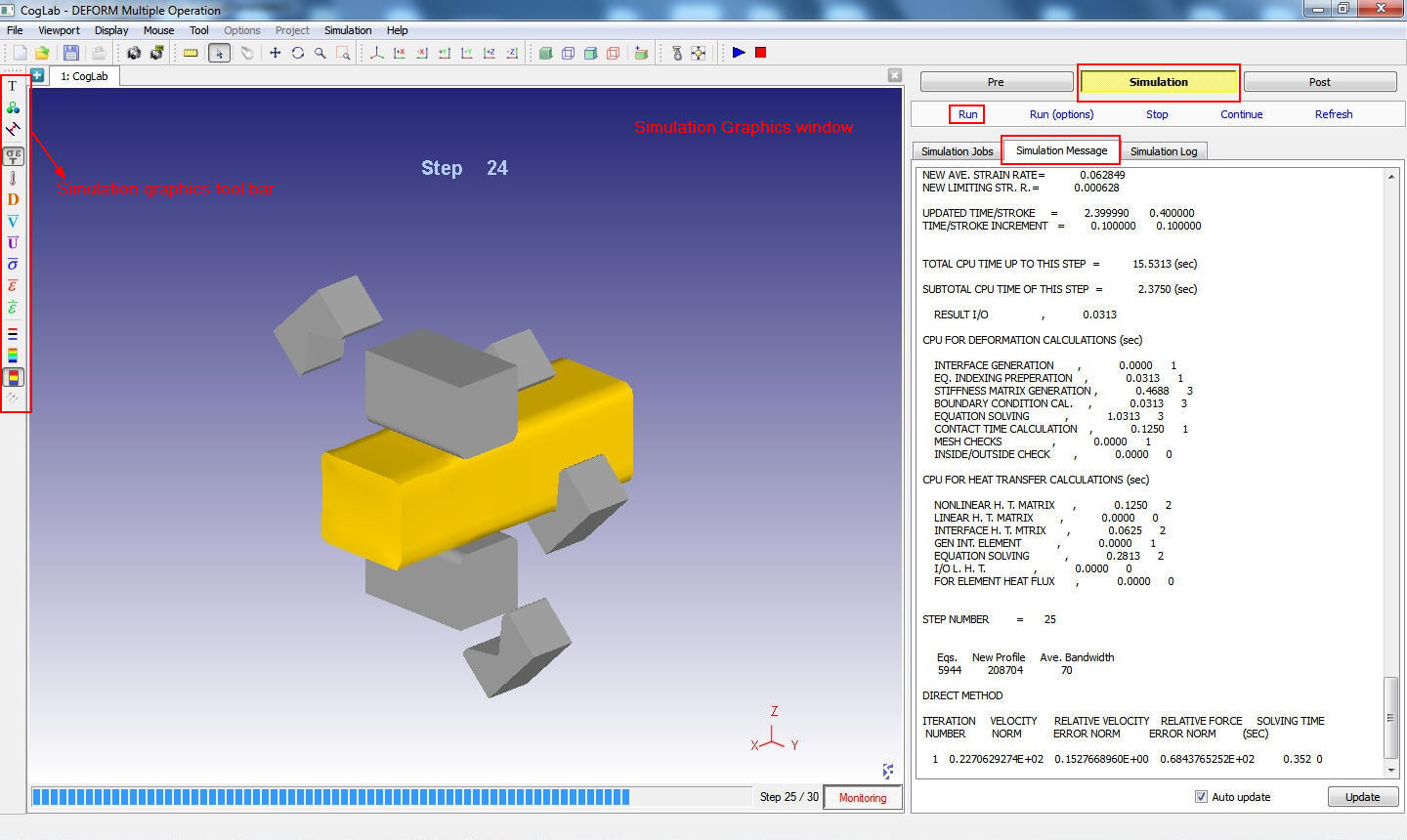
Simulation Mode

For cogging simulation, all simulation information of cogging while running will be written to ProblemID.MST file, ProblemID.MST file helps to run the cogging simulation sequentially each bite deformation and heat transfer operations as individual operations based on the settings in process window and pass table. ProblemID.MST controls the start and stop of each operation. For all operations, start and stop messages are showed in Message file. After the completion of the all operations, in Simulation Log file we will see message as “MULTIPLE OPERATION COMPLETED”.

Post Processing

When the simulation is complete, user can review the results by switching to Post mode using the button above the Simulation tool bar. (See Fig. 29.1.61.)

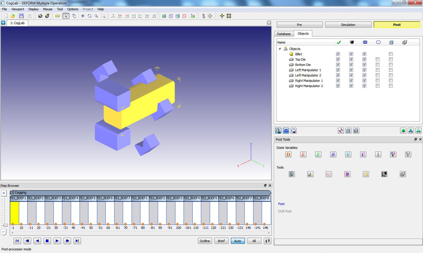
Post processor mode

Play through the Steps and see the Temperature distribution and Strain distribution by plotting the Temperature and effective strain State variables. (See Fig. 29.1.62.) The temperature change in dies can also be noticed as shown in Fig. 29.1.63.

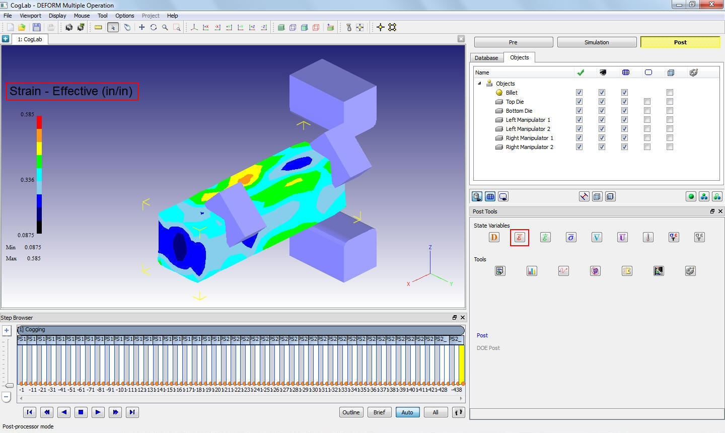
Strain Distribution in Billet

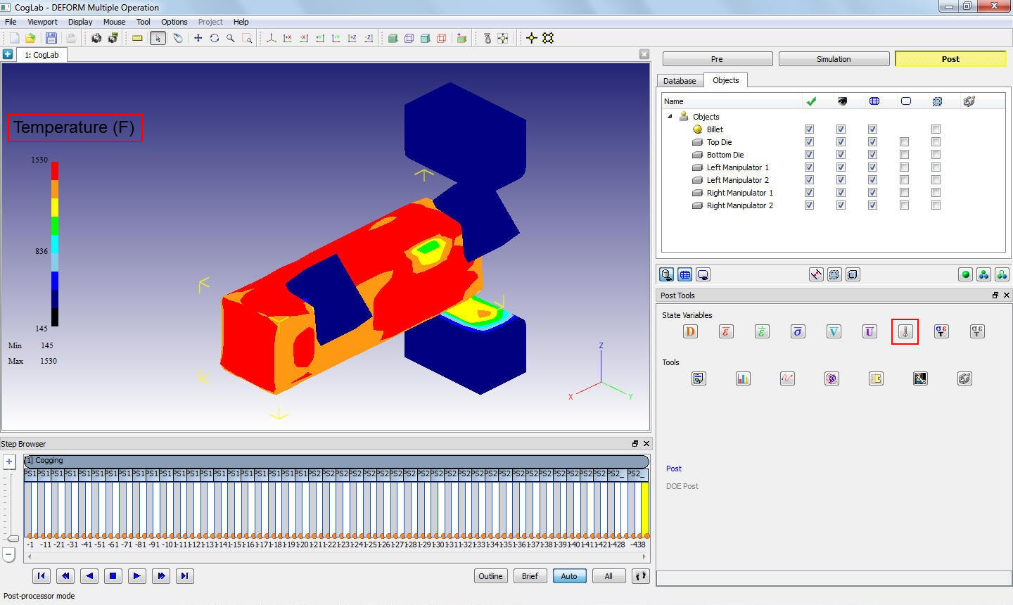
Temperature distribution in Billet and Dies

Related Topics:

Cogging Lab

6.1. Integrated Manufacturing Process Pre- Processor Layout

6.2. Integrated Manufacturing Process.Simulation layout

6.3. Integrated Manufacturing Proces Post - Processor layout

29. Introduction to Cogging