Tool Life Study Lab1
1.1. Introduction
1.2. Creating a New problem
1.2.1. Adding Tool life study
1.2.2. Objects definition
1.2.2.1. Top Die
1.2.2.2. Bottom Die
1.2.3.1. Data Extraction
1.2.3.2. Curve fitting
1.2.3.3. Simulation Controls
1.2.4. Fatigue
1.2.4.1. Cycle selection
1.2.4.2. Simulation controls
1.2.5. Generate Database
1.2.6. Running simulation
1.2.7. Post Processing
1.2.7.1 Tool Life Post
Introduction
Tool life impacts manufacturing cost. It is determined by many factors such as tool temperature, tool wear, tool fatigue and so on. In the Tool Life Module, we perform steady-state temperature, tool wear prediction and multi-step die stress calculation in the preprocessor which will be used for fatigue analysis in the postprocessor.
In this lab, we will be copying already simulated 2D Spike project that has a forming operation simulated over 5 cycles with tool wear calculation for dies.
Creating a New problem
On a Windows machine, go to the ![]() button, select DEFORM-v1x.xxx (.xxx indicates version number E.g. v14.0.2) and select DEFORM GUI Main v1x.x from the menu. The DEFORM GUI Main window will appear.
button, select DEFORM-v1x.xxx (.xxx indicates version number E.g. v14.0.2) and select DEFORM GUI Main v1x.x from the menu. The DEFORM GUI Main window will appear.
Create a new problem either by selecting File![]() **New Problem** or by clicking the New Problem
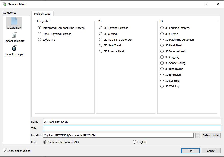
**New Problem** or by clicking the New Problem ![]() icon. The Problem Setup window will appear as shown in Fig. TLSL1.1. Select “Integrated Manufacturing Process “ radio button and Unit system as “SI “ using radio button. Define Problem Name as “2D_Tool_Life_Study “ and make sure the “Show option dialog” check box is turned on (if we do not turn on the “Show option dialog ” check box, then we will not get the New Project dialog in MO UI). Then click on
icon. The Problem Setup window will appear as shown in Fig. TLSL1.1. Select “Integrated Manufacturing Process “ radio button and Unit system as “SI “ using radio button. Define Problem Name as “2D_Tool_Life_Study “ and make sure the “Show option dialog” check box is turned on (if we do not turn on the “Show option dialog ” check box, then we will not get the New Project dialog in MO UI). Then click on ![]() button to open a new Problem using the Deform Integrated Manufacturing Process.
button to open a new Problem using the Deform Integrated Manufacturing Process.
Problem type selection window
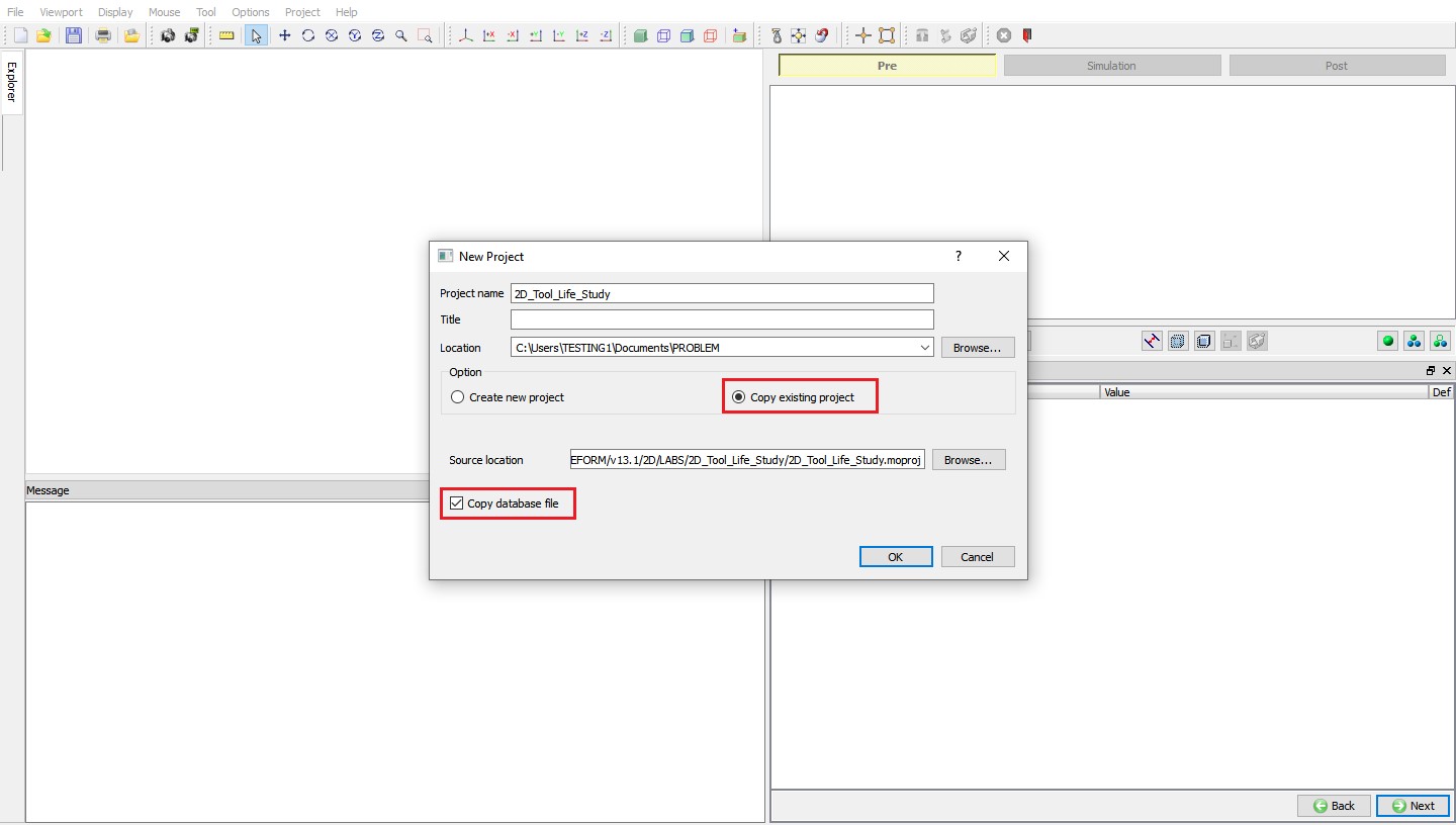
Multiple operation wizard will open with the New Project dialog as shown in Fig. TLSL1.2., at this point user will be prompted to specify a project name (system will create a separate folder with this project name) and title for this session. In this session we will use ‘2D_Tool_Life_Study ’ as the project name. We will import already simulated 2D project “2D_Tool_Life_Study” from 2D/LABS/ installation folder using “Copy existing Project” option.
Select “Copy existing project ” radio button in New Project dialog, then click on Source location and browse the “2D_Tool_Life_Study.moproj ” file from 2D\LABS\2D_Tool_Life_Study installation folder using ![]() button. Turn on “Copy database file ” check box as shown in Fig. TLSL1.2. so that database file is copied along with the project file. Click on
button. Turn on “Copy database file ” check box as shown in Fig. TLSL1.2. so that database file is copied along with the project file. Click on ![]() to continue to open the operation. The loaded MO project is as shown in Fig. TLSL1.3.
to continue to open the operation. The loaded MO project is as shown in Fig. TLSL1.3.
MO wizard New Project with Copy existing project option
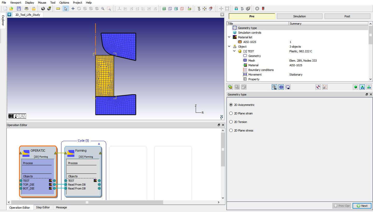
Copied 2D_Tool_Life_Study project Loaded in MO wizard
Adding Tool life study
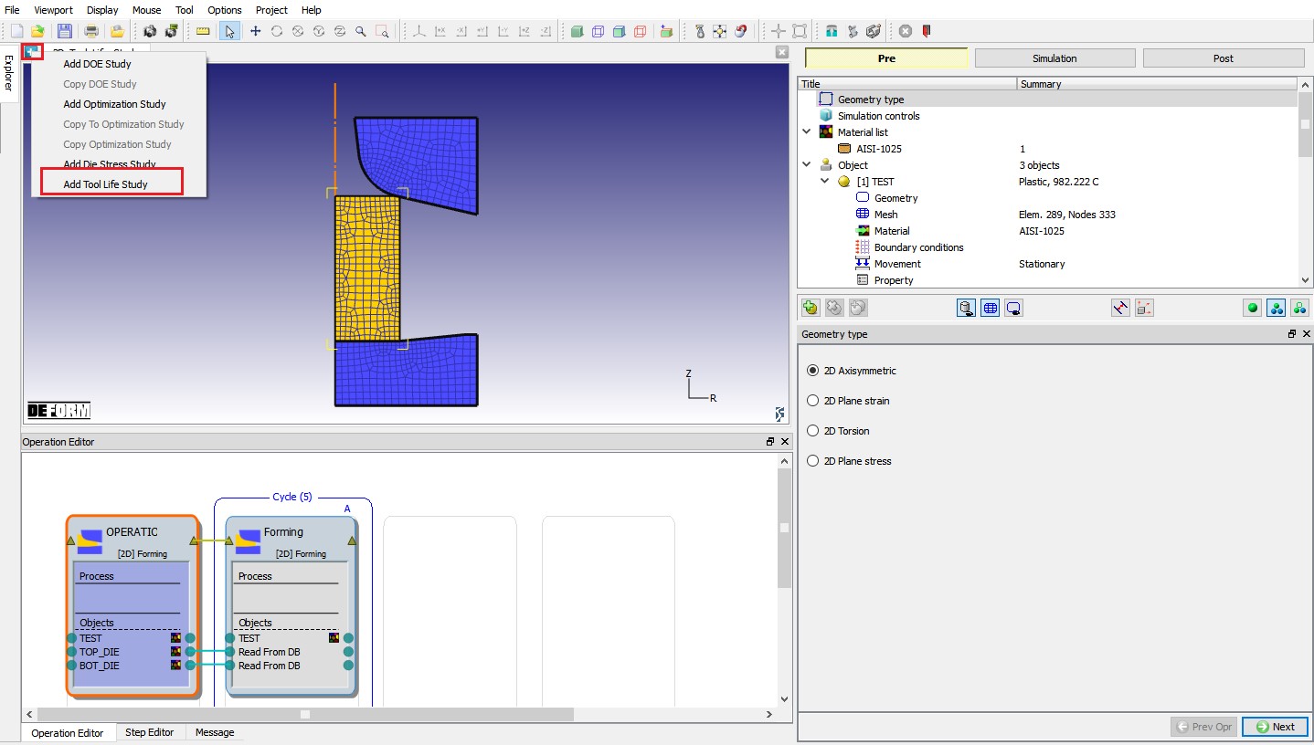
Click on ![]() (Add new study) button and select “Add Tool Life Study ” option as shown in Fig. TLSL1.4. Added Tool life study is as shown in Fig. TLSL1.5.
(Add new study) button and select “Add Tool Life Study ” option as shown in Fig. TLSL1.4. Added Tool life study is as shown in Fig. TLSL1.5.
Adding Tool life study
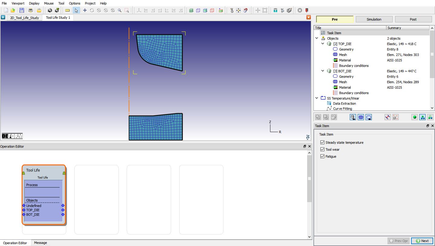
Added Tool life study operation in MO.
The die objects are loaded from Forming operation. There are three options in Task Item,
-
Steady state temperature,
-
Tool Wear and
-
Fatigue
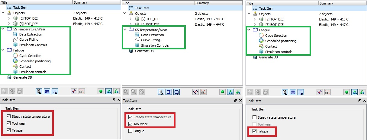
The first two options, Steady state temperature and Tool Wear, will predict the steady-state temperature and tool wear based on the history data from Forming operation. The Fatigue option will activate multiple step die stress study and use the stress data to perform Fatigue analysis in the post processor. In this example, we will select all the three options. Notice that as we update the task item options, the operation tree will be also updated, as shown in Fig. TLSL1.6.
In Task Item, make sure Steady state temperature, Tool Wear and Fatigue check boxes are in checked status and then click ![]() to Object page.
to Object page.
Note :
• The dies which are studied for Steady-State temperature and Tool wear must be meshed in nominal setup, for Fatigue-only task mesh in nominal setup is not required.
• “Define model to calculate tool wear” checkbox must be turned on in inter-object relations of nominal setup for dies whose tool wear will be studied.
• Tool life study can be executed only for one forming operation and that forming operation must be in cycle in nominal setup to execute Tool life study.
Task Item Update
Objects definition
We will use all dies object from “Forming” operation for tool life study in this lab, so click ![]() to Top Die page.
to Top Die page.
Top Die
Fig. TLSL1.7. shows the object page of top die. For each object, we also have three options – steady state temperature, tool wear and fatigue. This allows us to choose if a specific analysis is needed/excluded for the current object. In this lab, we will keep the default selection and perform all the three tasks for each die object. Click ![]() until BCC page.
until BCC page.
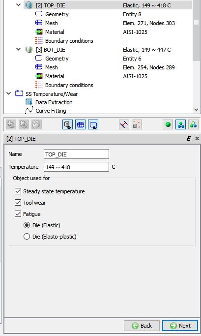
Top Die object page
Top Die Boundary Conditions
Apply Velocity boundary condition (Vy=0) for Top die on Top surface as shown in Fig. TLSL1.8. Then click ![]() until Bottom Die page.
until Bottom Die page.
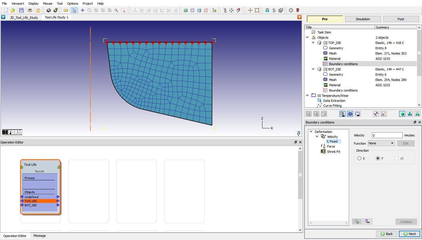
Assigned Velocity (Vy=0) boundary condition for Top die
Bottom Die
In this lab, we will keep the default selection and perform all the three tasks for each die object. Click ![]() until BCC page.
until BCC page.
Bottom Die Boundary conditions
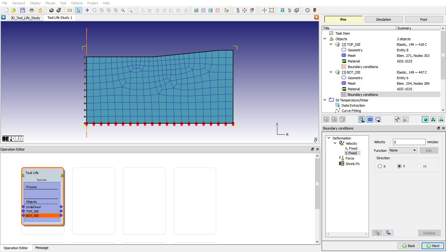
Apply Vx=0 velocity boundary condition on the symmetry surface and Vy=0 velocity boundary condition for Bottom die on Bottom surface as shown in Fig. TLSL1.9. Then click ![]() until SS Temperature/Wear page.
until SS Temperature/Wear page.
Assigned Velocity boundary condition for Bottom die
SS Temperature/Wear
Now we are going to setup the steady state temperature and tool wear simulation. The idea is to extract heat flux/wear from the contact area with workpiece and fit the data using exponential functions. And then, impose the fitted data on the die objects and run heat transfer simulation for a sufficiently longer period until the convergence of thermal state.
Data Extraction
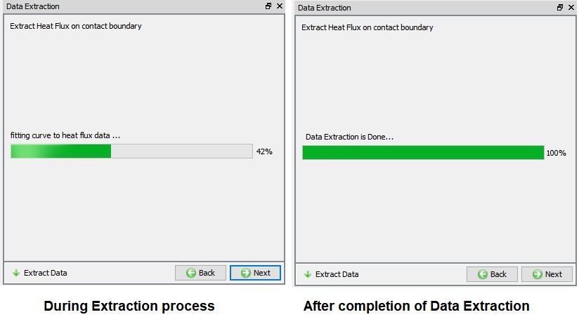
Click on Data Extraction from Operation tree, click on ![]() button to start extracting heat flux/wear from the contact area with workpiece. The progress bar in Data Extraction page shows the progress of extracting heat flux and wear from the contact area of the die objects. Once the extraction and fitting are complete, we can see the fitted coefficients in the curve fitting page. Click
button to start extracting heat flux/wear from the contact area with workpiece. The progress bar in Data Extraction page shows the progress of extracting heat flux and wear from the contact area of the die objects. Once the extraction and fitting are complete, we can see the fitted coefficients in the curve fitting page. Click ![]() to Curve Fitting page.
to Curve Fitting page.
Data Extraction page
Curve fitting
We can check the contacted area and the fitted curve by clicking on the ![]() icon as shown in Fig. TLSL1.11. Meanwhile, Intermediate and final result files will be generated and saved in Operations/Task00004 directory, which includes two subfolders – HeatFlux and ToolWear storing the results for heat flux extraction and tool wear extraction respectively, and OutputForPredict.KEY which is the object keyword file containing the fitted coefficients.
icon as shown in Fig. TLSL1.11. Meanwhile, Intermediate and final result files will be generated and saved in Operations/Task00004 directory, which includes two subfolders – HeatFlux and ToolWear storing the results for heat flux extraction and tool wear extraction respectively, and OutputForPredict.KEY which is the object keyword file containing the fitted coefficients.
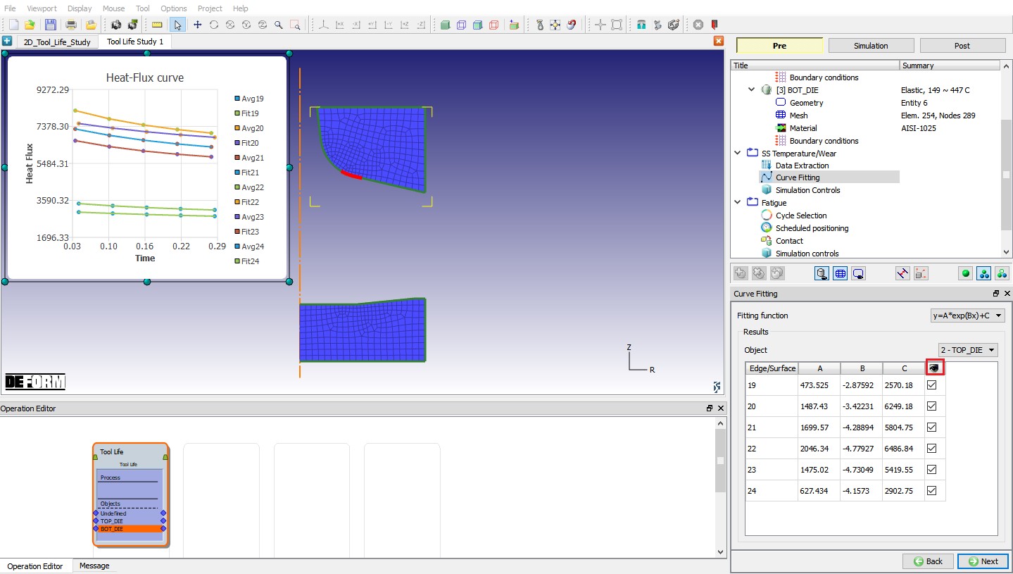
Curve Fitting page
Simulation Controls
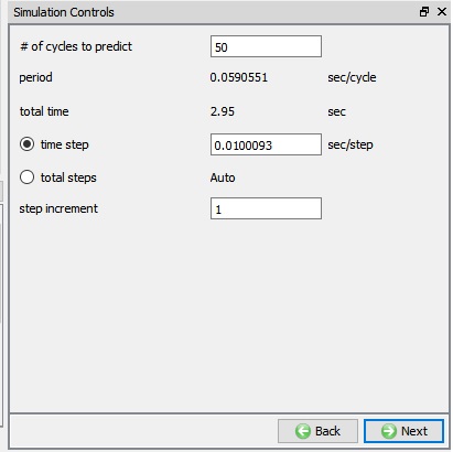
We set up the simulation control parameters for steady state temperature prediction, which involves heat transfer simulation on the die objects with heat flux BCC using the fitted coefficients. As shown in Fig. TLSL1.12. we only need to define three parameters - # of cycles to predict (total time will be calculated automatically based on process time of the forming operation which is in cycle), either time step or total steps and step increment. The default # of cycles to predict is set to be 10 times of the number of cycles in the forming operation, which is 50 in this case. In this lab, we will use # of cycles to predict as 50 with timestep as 0.0100093 sec/step and step increment as 1 as shown in Fig. TLSL1.12.
Temp Simulation controls page
Fatigue
The final task in the preprocessor is Fatigue, which is essentially setting up die stress calculation at multiple steps from cycle operation. The first step is to select cycles from the forming operation to perform die stress calculation (see Fig. TLSL1.13.). We can either select the last cycle from the database, all cycles or select cycles incrementally. We will also need to set up simulation control parameters for die stress calculation (see Fig. TLSL1.14.).
Cycle selection
Select “Cycle**Selection** ” under Fatigue from Operation tree, make sure by default “Lastcycle ” is selected as shown in Fig. TLSL1.13. If not selected, then select “Lastcycle ” radio button. Click ![]() until Simulation controls page.
until Simulation controls page.
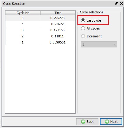
Cycle selection page
Simulation controls
In Simulation controls, we will use default Number of simulation steps as 1 , Step increment to save as 1 and Time per step as 1e-06 as shown in Fig. TLSL1.14. Click ![]() to Generate DB page.
to Generate DB page.
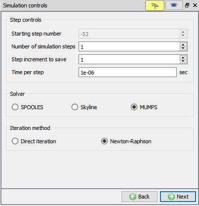
Fatigue- Simulation controls page
Generate Database
As we click on ![]() to Generate DB, we will get Data Extraction popup while loading generate DB page as shown in Fig. TLSL1.15. Select
to Generate DB, we will get Data Extraction popup while loading generate DB page as shown in Fig. TLSL1.15. Select ![]() in the popup since we had already done the data extraction.
in the popup since we had already done the data extraction.
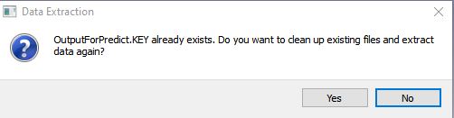
Data Extraction popup
Click on ![]() action label to check if there are any errors or warnings that would stop DB generation. Generate the database if there are no errors or warnings by clicking
action label to check if there are any errors or warnings that would stop DB generation. Generate the database if there are no errors or warnings by clicking ![]() action label (see Fig. TLSL1.16.).
action label (see Fig. TLSL1.16.).
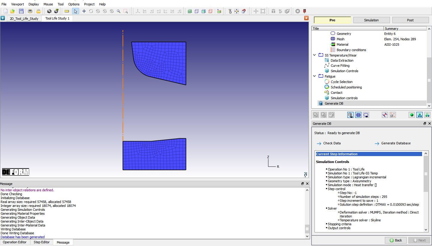
Generate Database window
Running simulation
Once the database has been generated, switch to the Simulation mode by clicking on ![]() button above the operation tree. Click on the
button above the operation tree. Click on the ![]() action label to open the Run Options dialog as shown in Fig. TLSL1.17. Use the default Continue Run option to select “Continue from the last step ” (from step -1) option and then select the Simulation mode as Interactive and click on
action label to open the Run Options dialog as shown in Fig. TLSL1.17. Use the default Continue Run option to select “Continue from the last step ” (from step -1) option and then select the Simulation mode as Interactive and click on ![]() button to run the simulation.
button to run the simulation.
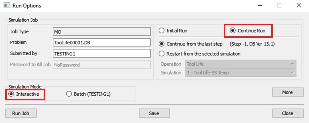
Run Options Popup
The progress of the simulation can be monitored as it is running by looking at the Simulation Message tab and Simulation Graphics from the Graphics display region in Simulation mode. If ![]() option is checked in Simulation Message tab, which is the default setting, the Message file will refresh automatically.
option is checked in Simulation Message tab, which is the default setting, the Message file will refresh automatically.
The Message file provides information about which simulation step the simulation is currently on and information regarding how well the simulation is running as shown in Fig. TLSL1.18.
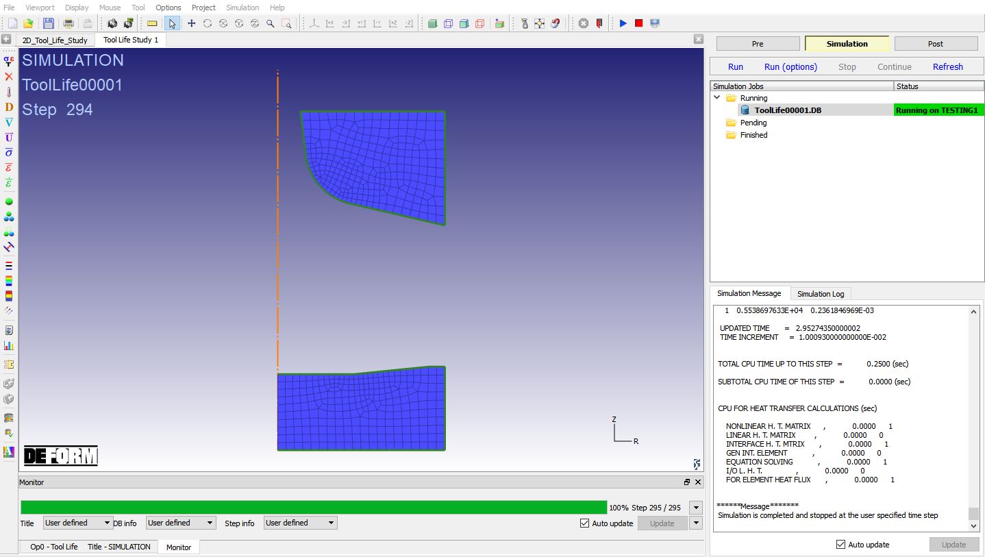
Simulation mode
Post Processing
After the simulation is completed, click on ![]() tab to visit MO post processor. The simulated results can be seen in Post ( Fig. TLSL1.19.). It contains two parts, one is the temperature history from running heat transfer with imposed heat flux BCC and the other is the die stress.
tab to visit MO post processor. The simulated results can be seen in Post ( Fig. TLSL1.19.). It contains two parts, one is the temperature history from running heat transfer with imposed heat flux BCC and the other is the die stress.
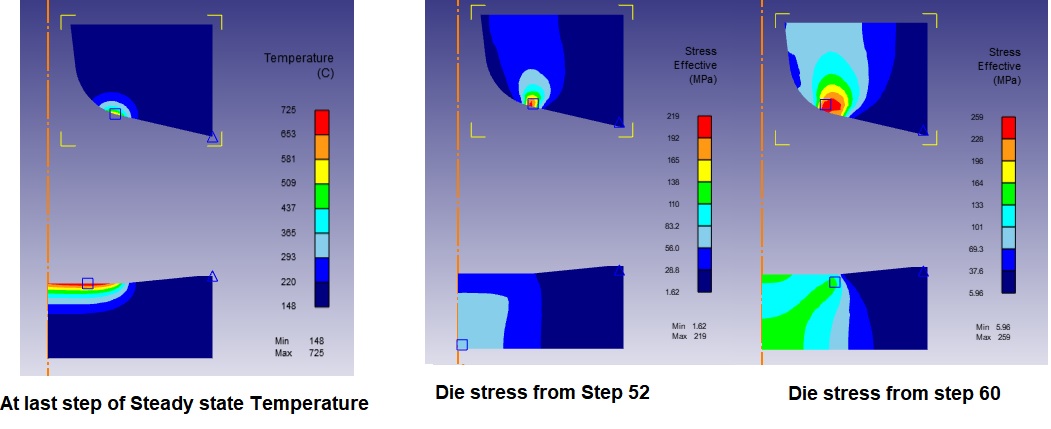
The steady state heat transfer analysis and tool wear analysis steps are grouped under simulation name SS Temp. Here the simulation name Fatigue-Step52 means the die stress result from step 52 in the forming operation. There is a highlighted toolbox used for fatigue analysis based on the calculated die stress data. Fig. TLSL1.19. summarizes the simulation results of temperature and die stresses from SS Temperature prediction and multi-step die stress study. We take the last step from heat transfer simulation as the steady-state temperature and impose it on the die objects while running die stress calculation. Note that if we select fatigue as the only task, we will impose the temperature profile from the corresponding steps from the forming operation as initial temperature.
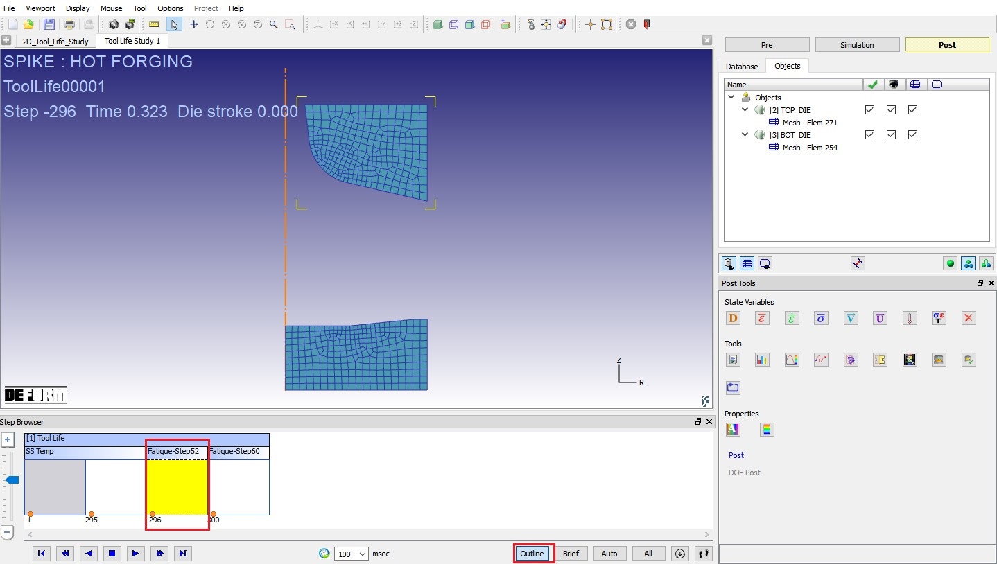
MO Post – Fatigue -Step52
Click on ![]() button in Step browser, then Play animation from first step with Temperature State Variable to observe the die temperature as they approach steady state.
button in Step browser, then Play animation from first step with Temperature State Variable to observe the die temperature as they approach steady state.
Simulation Results
Tool Life Post
Tool Life Post is used for analysis of steady-state temperature and tool wear results, as well as fatigue life prediction of dies. From MO post, we can access Tool life post by clicking on ![]() button as shown in Fig. TLSL1.19. Tool life post is opened as shown in Fig. TLSL1.21
button as shown in Fig. TLSL1.19. Tool life post is opened as shown in Fig. TLSL1.21
SS Temp & Wear: By selecting this option, we can plot the results for SS Temp & Wear operation (See Fig. TLSL1.21.). Under this option, we can plot Tool temperature, Tool wear depth, tool wear rate and Worn geometry output for selected Cycle no.
We can select the different cycle number under Cycle section by dragging sliding bar or by entering the respective cycle number in input field. Once you enter the cycle number, user can select one of tool wear results to view the results in display, Fig. TLSL1.22 shows Tool Wear depth at Cycle 40.
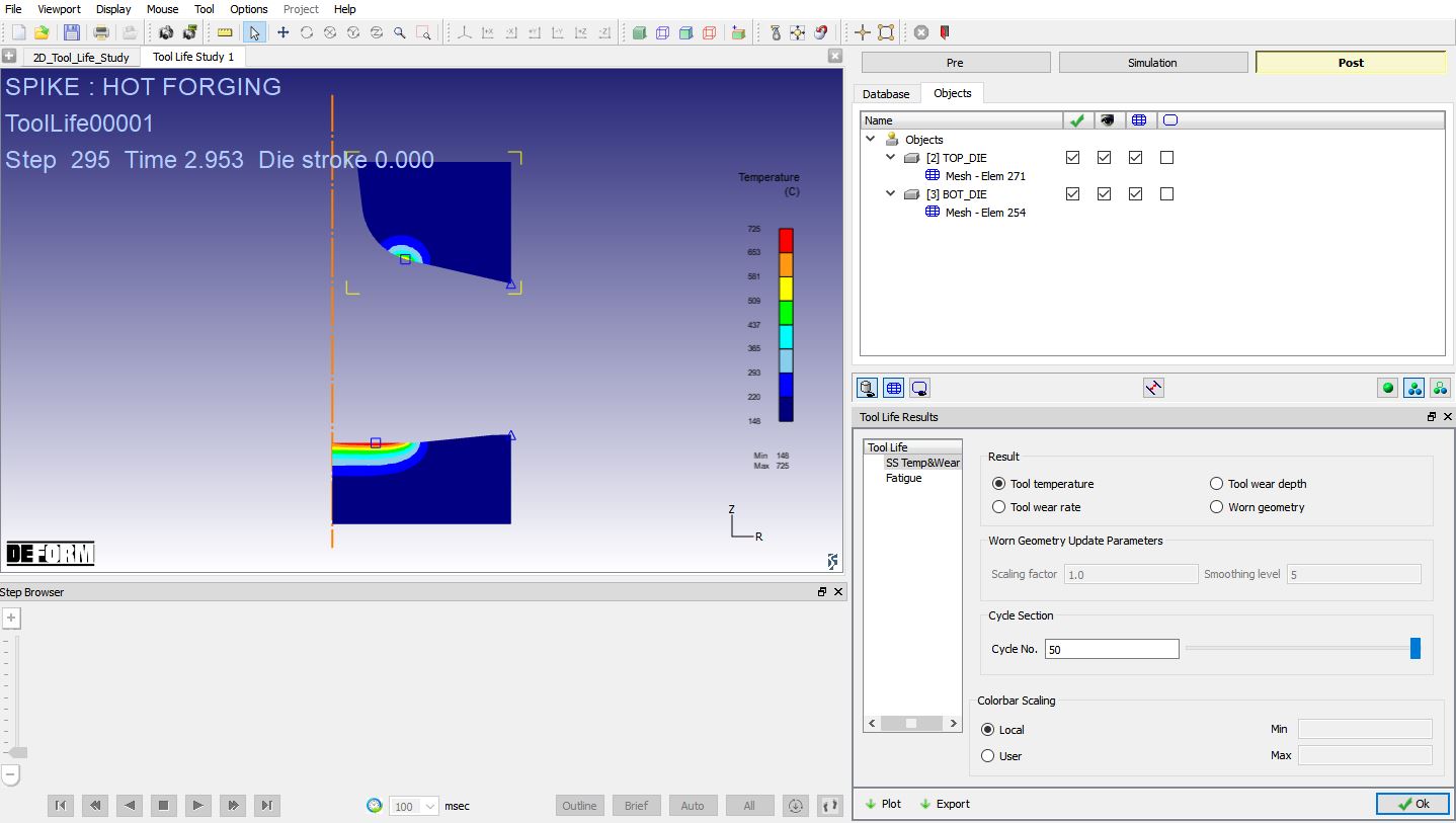
Tool life results for SS Temp & Wear
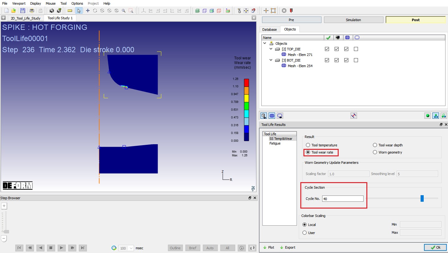
Tool wear rate result at Cycle 40
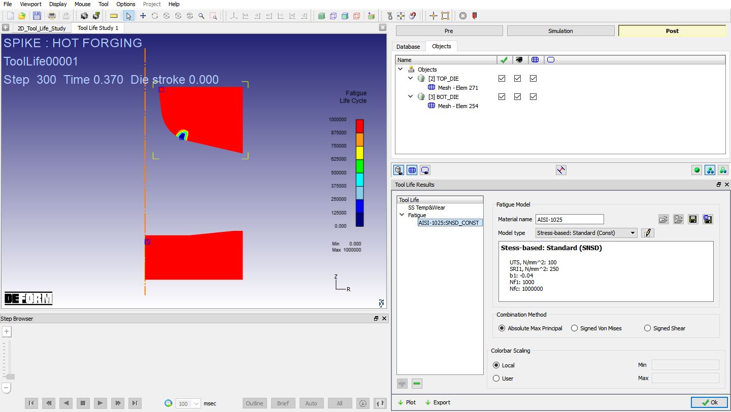
Fatigue : By selecting this option, we can plot the results for Fatigue operation (See Fig. TLSL1.23.). Initially there will not be any fatigue model in the list. We can add fatigue model by clicking the ![]() button. The model named “AISI-1025:SNSD_CONST ” is added, where AISI-1025 stands for the material name and SNSD_CONST stands for the stress-based standard model. We can observe that a Stress-based standard model is selected as Model type. We can define the model parameters by clicking the
button. The model named “AISI-1025:SNSD_CONST ” is added, where AISI-1025 stands for the material name and SNSD_CONST stands for the stress-based standard model. We can observe that a Stress-based standard model is selected as Model type. We can define the model parameters by clicking the ![]() button and a function editor will pop up. The parameters we defined for this model can be found in Fig. TLSL1.24. The other way to add fatigue model is by loading model files from a user directory or Fatigue library. Note that we need to be in Fatigue page to enable the load buttons (see Fig. TLSL1.25.). The model file has the same format as keyword file, where the keyword is followed by its value.
button and a function editor will pop up. The parameters we defined for this model can be found in Fig. TLSL1.24. The other way to add fatigue model is by loading model files from a user directory or Fatigue library. Note that we need to be in Fatigue page to enable the load buttons (see Fig. TLSL1.25.). The model file has the same format as keyword file, where the keyword is followed by its value.

Tool Life post – Fatigue output
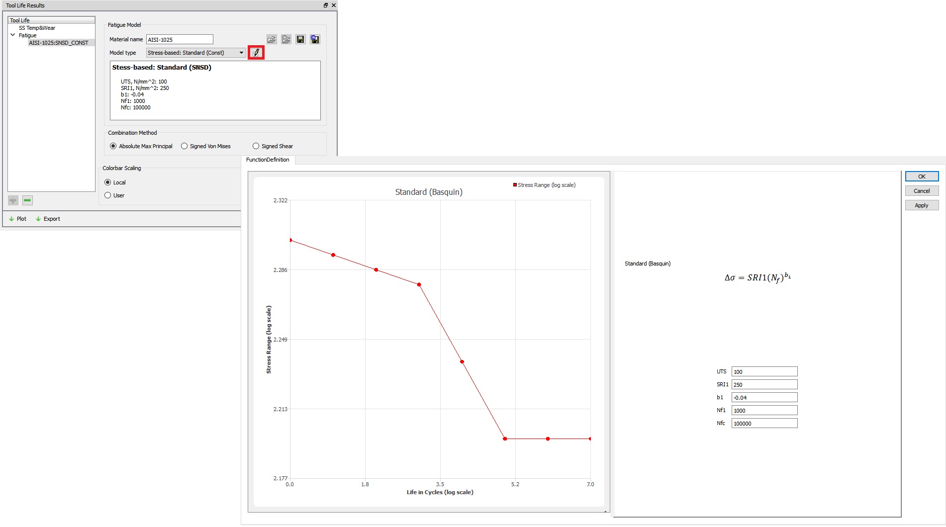
Fatigue model definition
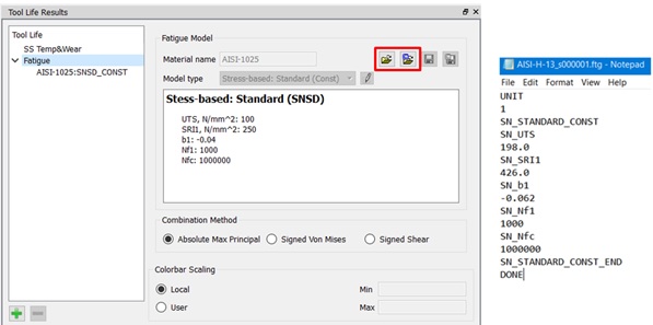
Loading model file
Once the model is defined, we can see the fatigue life prediction plot by selecting either Absolute Max principal or Signed Von Mises or Signed Shear as the combination method with model and clicking the ![]() button. The result is shown in Fig. TLSL1. 26.
button. The result is shown in Fig. TLSL1. 26.
Fatigue Life Plot