2D HT Lab1: Modeling of a Heating Operation with Phase Transformation

1.1. Creating a New Problem

1.2. Open Operation and Select geometry

1.3. Loading the material properties

1.4. Adding Objects

1.5. Creating Object1

1.6. Creating Object2

1.7. Inter-Object Definition

1.8. Setting Simulation Controls

1.9. Generate Database

1.10. Running a Simulation

1.11. Post processing the Results

1.12. Exiting the MO wizard

Creating a New problem

On a Windows machine , go to the button select DEFORM-v1x.xxx (.xxx indicates version number E.g. v14.0.2) and select DEFORM GUI Main vxx.xx from the menu. The DEFORM GUI Main window will appear as shown below Fig. 2DHTML1.1.)

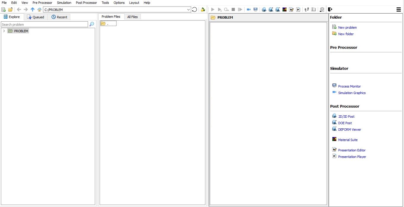
DEFORM GUI main window

Create a new problem either by selecting File **New Problem** or by clicking the New Problem icon. The Problem Setup window will appear as shown in Fig. 2DHTML1.2. Select “ Integrated Manufacturing Process “ radio button and units system as “SI “ using radio button. Define Problem Name as “Gear_Blank “ and click on button to open a new Problem using the Integrated Manufacturing Process.

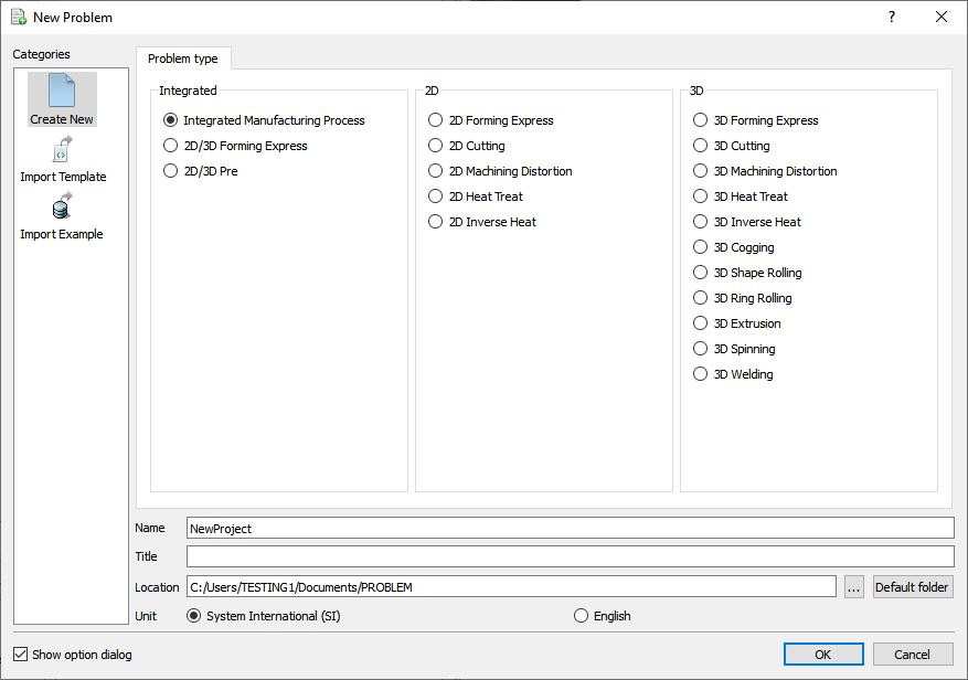
Problem type selection window

MO wizard will open along with project naming window, defined problem name is updated as ‘Gear_Blank ’ as the project name and selected unit system updated. Select Firstoperation as[2D] Forming as shown in Fig. 2DHTML1.3. and click on to add project.

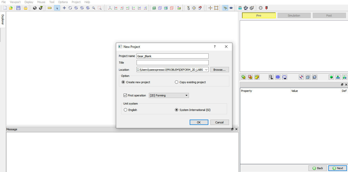
MO wizard New project

Open Operation and Select Geometry Type

As we selected the first operation while adding project, first operation will open automatically. In this lab we are using Plane Strain geometries, So select 2D Plane strain radio button in geometry type page as shown in Fig. 2DHTML1.4., then click on .

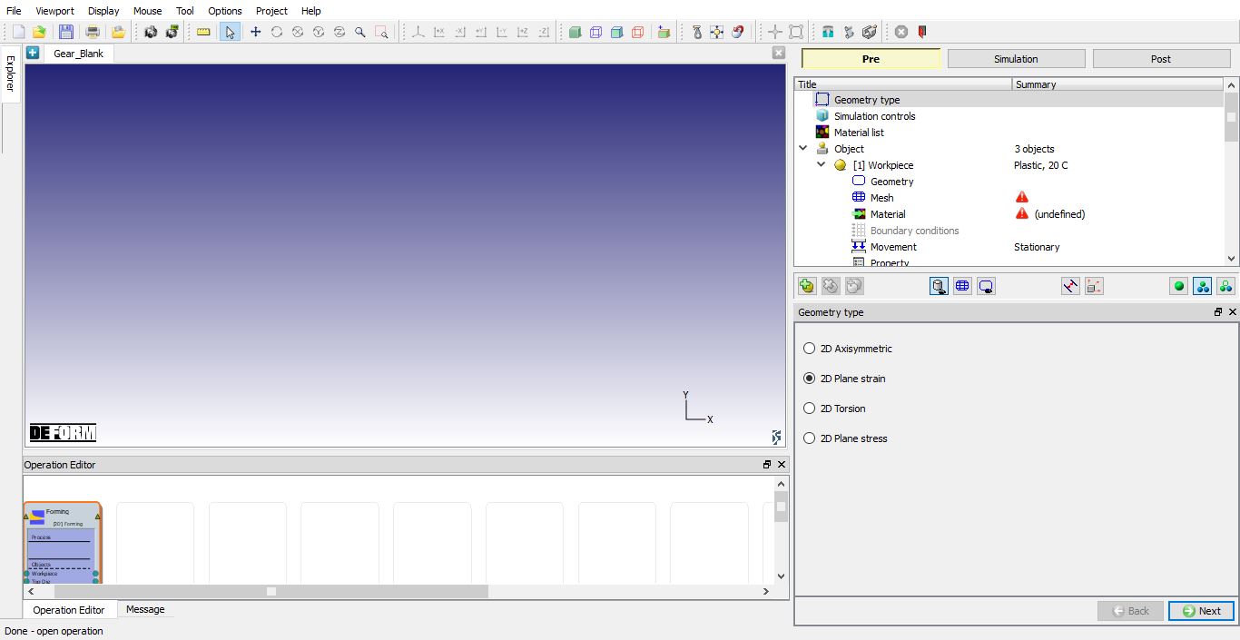
Added 2D Forming operation into Operation Editor and selected plane strain geometry type

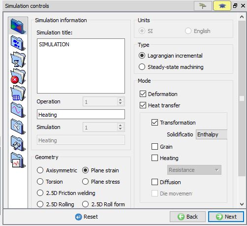
In simulation controls guided mode, under Sim Mode tab, Turn on Deformation , Heattransfer and Transformation as shown in Fig. 2DHTML1.5. Click on .

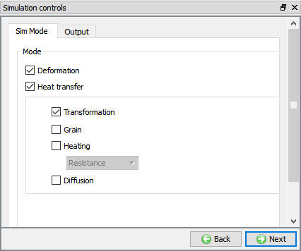
Simulation controls in Guided mode

Loading the Material Properties

In Material list Window, click on to Load material data from Library and select the category Steel and load material “JIS-S45C (Heat Treatment) ”. This material is a mixture material with three components (phases): Austenite, Pearlite, and Martensite. These components combine to define the properties of the mixture material, using the weighted-average mixture rule based on volume fractions of each component. Therefore, for each phase, the elastic, plastic and thermal data are defined. To help users better understand the requirements on material data, we recommend users to review at least the flow stress data, Young’s modulus, and thermal conductivity of each phase. (See Fig. 2DHTML1.6.)

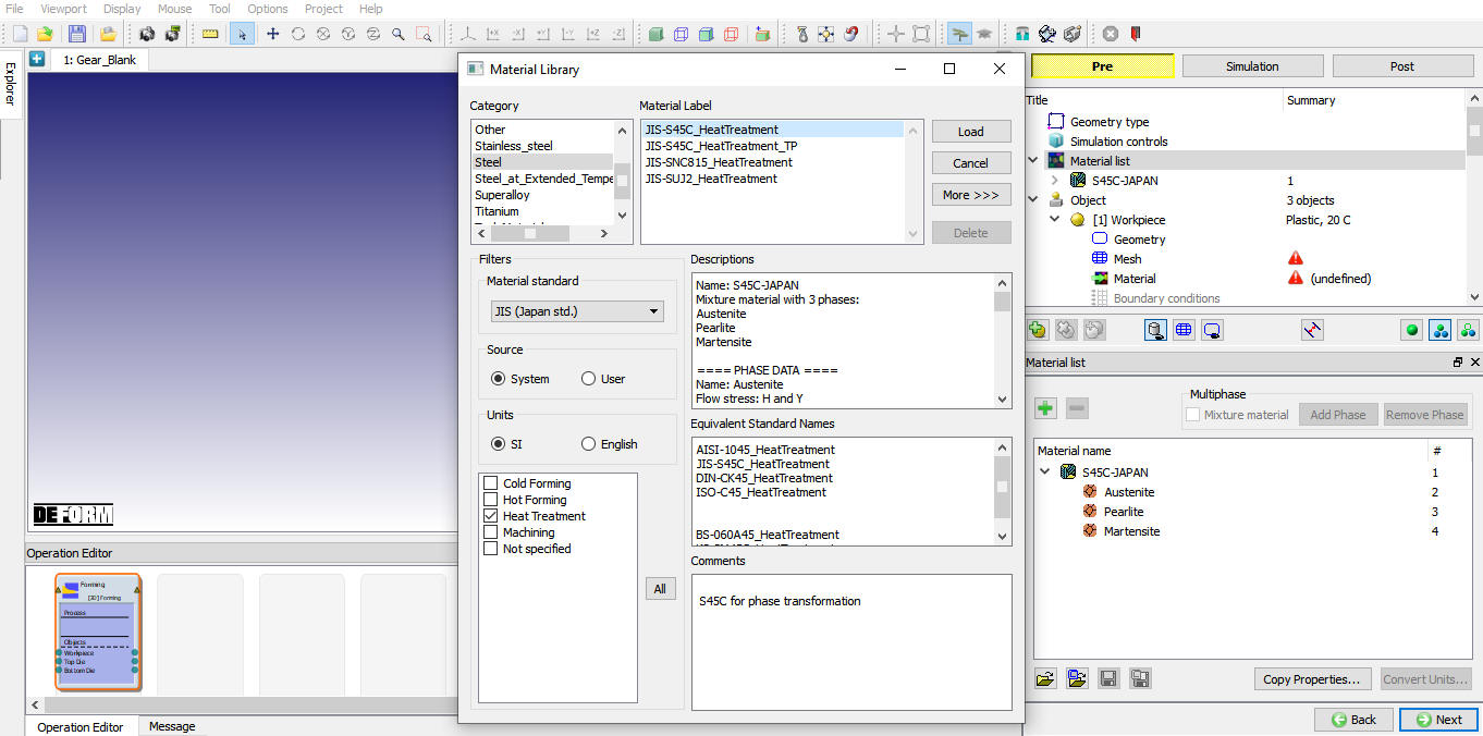
Material definition window

The relations between these phases are defined in the Phase Transformation Dialog, which can be accessed by clicking the Transformation button. For each relation, there is a kinetics model for determining the rate of phase transformation. Related properties include latent heat and volume change, etc. Click on unitl Object page.

Adding objects

Now by default 3 Objects will be added to Objects list, So delete last objects by clicking the delete object button , two objects in the list named as Workpiece and Top die as shown in Fig. 2DHTML1.7. Click on button to go to Workpiece page.

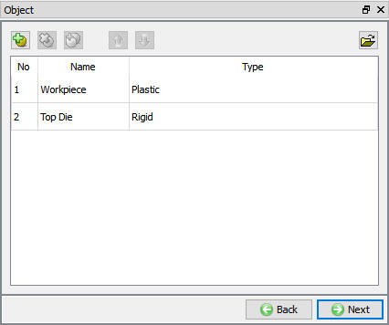
Adding Objects

Creating Object1

As you enter the Workpiece page, change the Object Name to Gear and select the object type to Elasto-Plastic as shown in Fig. 2DHTML1.8. Assign Temperature as 20°C to the object. Click on .

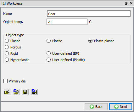
Workpiece object definition

Importing Geometry

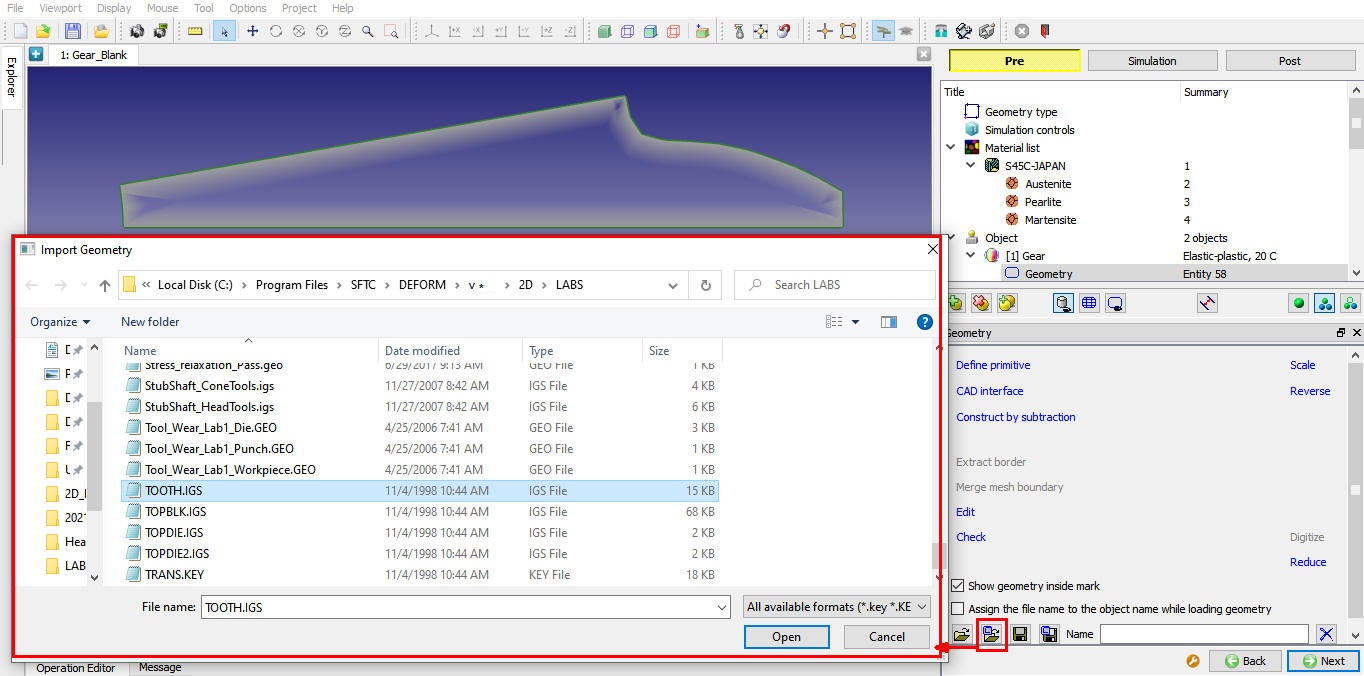
In Geometry page, click on import geometry from library option () and import the TOOTH.IGS file from DEFORM installed folder \2d\LABS directory as shown in Fig. 2DHTML1.9. Use action label to ensure that the geometry is legal. Click on to Mesh page.

Importing geometry file

Meshing the object

Switch to Expert mode by clicking on (Switch to expert mode) icon from the tool bar. Expert mode will provide more options for detailed settings.

In Mesh page, Select Weighing factors tab, set the boundary curvature - weightingfactor to 1.0 while leaving the other weighting factors unchanged as shown in Fig. 2DHTML1.10.

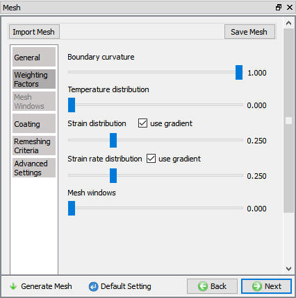
Weighing Factor window

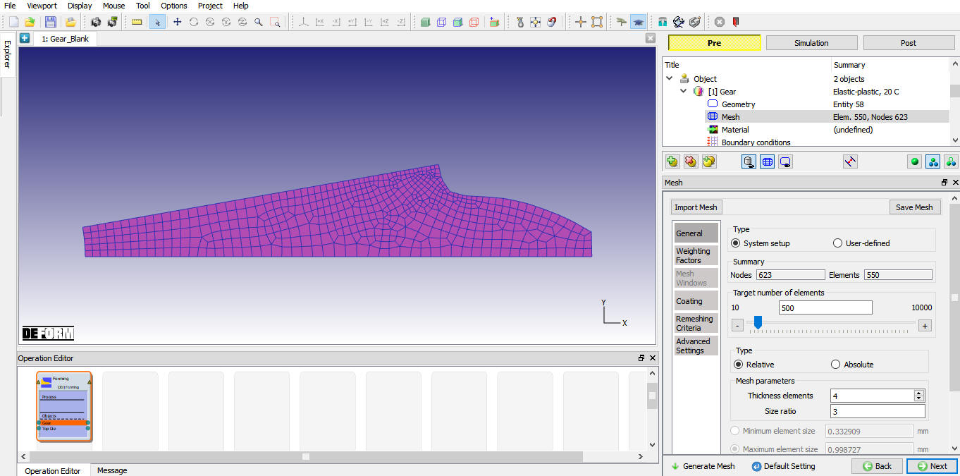
Select General tab, Define Target number of Elements as 500 , set the number of thickness elements to 4 and the sizeratio between elements to 3. After changing these settings, click on . Click on to object material page.

Defining and generating mesh

Again we can see the object material and we can edit material properties by clicking the option. Select the material in the list to add the material to object. Click on to go to Boundary conditions page.

Assigning Boundary Conditions

Select Vy=0 Velocity boundary condition on the bottom surface of the Gear as shown in Fig. 2DHTML1.12.

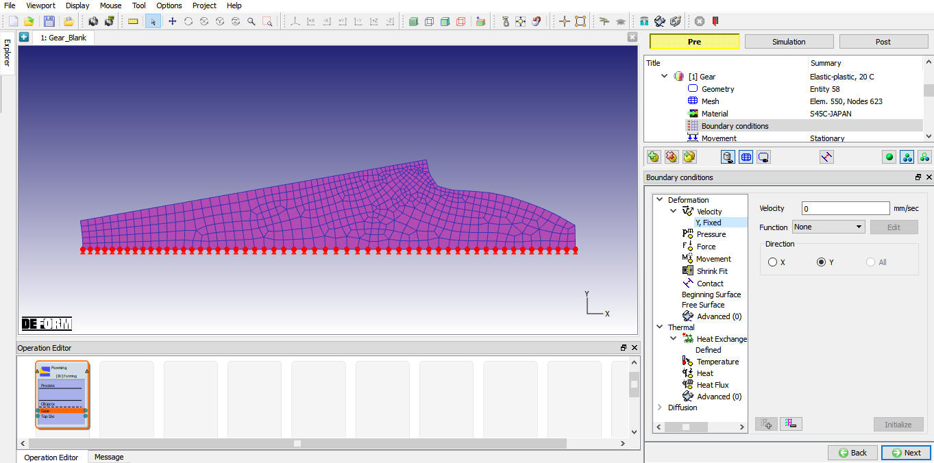
Gear tooth section with zero vertical velocity boundary conditions

Set the thermal boundary conditions to Heat Exchange with Environment for the outside part of the tooth and the bore (inner) section as shown in Fig. 2DHTML1.13.

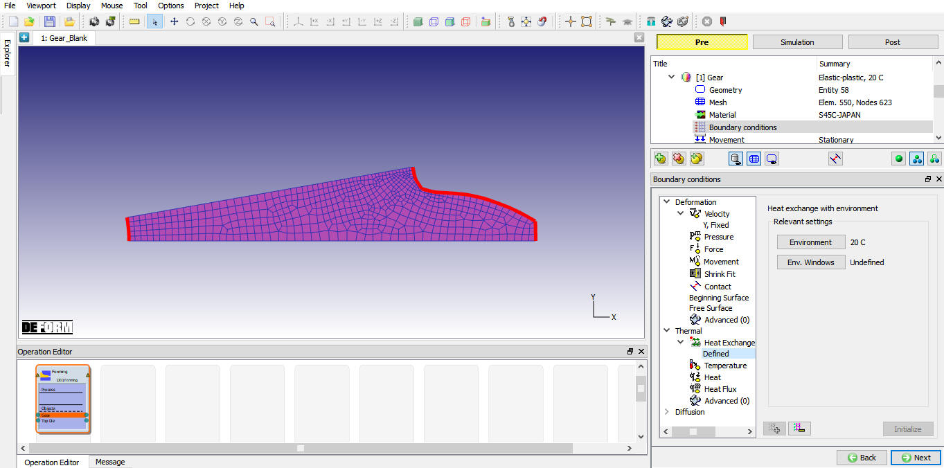
Gear Tooth section with Heat Exchange BCC

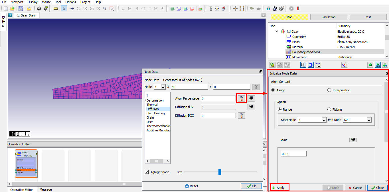
Select Objectnodes button, Node data window will open. In this dialog, click on Thermal tab check that the temperature is set to 20°C. In addition, click on Diffusion tab and initialize the AtomPercentage of all nodes to 0.14. as shown in Fig. 2DHTML1.14. Click the Plot variable button to confirm the state variables you just initialized. Click on to exit the dialog.

Diffusion Atom percentage data definition in Node data window

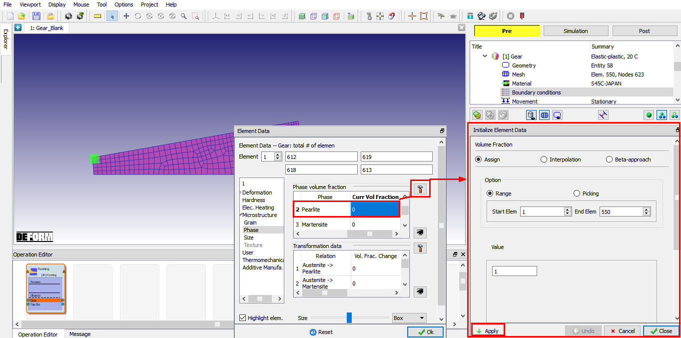
Click on the ObjectElement **icon. Element data dialog will open. In this dialog, click on **Microstructure , under that select Phase Transformation tab and initialize the Curr. Vol. Fraction of Pearlite to 1.0 for all elements as shown in Fig. 2DHTML1.15. Click to exit the dialog.

Phase Transformation data definition in Element data window

Note : The sums of all phase volume fractions must be equal to unity for each element. Otherwise the dialog will not accept the inputs.

Click on until Top Die page.

Creating Object2

As you enter the Top Die page, change the name of this object to Plane , make sure the object type is Rigid. (See Fig. 2DHTML1.16.)

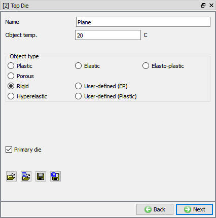
Top Die window

Import geometry

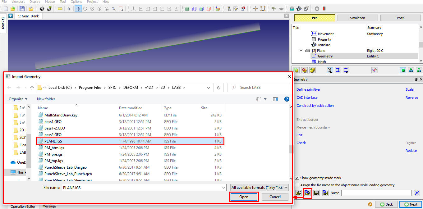
In Geometry page, click on import geometry from library option () and import the PLANE.IGS file from DEFORM installed folder \2d\LABS directory as shown in Fig. 2DHTML1.17. Use action label to ensure that the geometry is legal.

Importing Geometry

The purpose of this object is to serve as a plane of symmetry where no material may cross. The key to making this act as a true plane of symmetry is to set the interface heat transfer to zero, the friction to zero and the placing a no separation criteria between the two objects. These parameters will be prescribed later.

As objects are positioned by default, click on until Contact page.

Inter-Object Relations

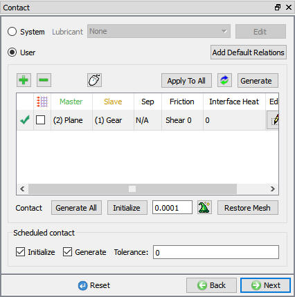
Select User type contact and click on button, define slave/master relationship between Plane to Gear as shown in Fig. 2DHTML1.18.

Inter-Object Window

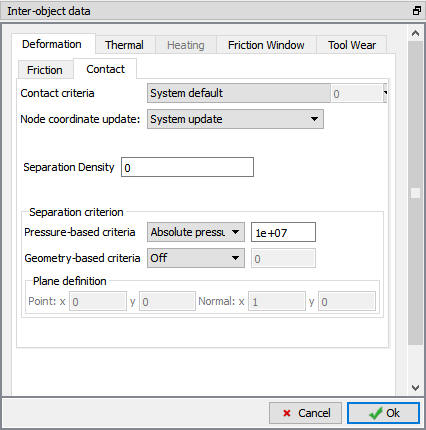
Select the Plane and Gear relationship and click the button to modify the contact conditions. Under Contact tab, set the separation criteria to AbsolutePressure and set the value to 1e+07 as shown in Fig. 2DHTML1.19. This prevents the gear tooth from losing contact with the symmetry plane. Click on to exit the Inter-Object Data Definition window.

Inter-Object deformation data definition window

Use icon to determine a suitable contact tolerance (a value of about 0.00126” will be calculated) , then click on button to generate contact.

Click on until Step page.

Setting Simulation Controls

Select Main tab, Change the Operation Name to Heating as shown in Fig. 2DHTML1.20.

Simulation controls main Tab in expert mode

Select Simulation Steps tab, Enter the number of simulation steps to 10000. Step Increment to save as every 10 steps as shown in Fig. 2DHTML1.21.

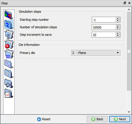
Defining Simulation steps

SelectStep Increment tab, Set solution Step Definition to Constant Temperature. Specify Initial/Minimum time step as 0.1 seconds per step and Max Temperature Change per Step should be set to 5 C. Max Temperature time step to 20 seconds per step. (see Fig. 2DHTML1.22.)

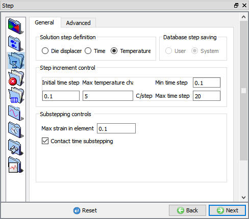
Step Increment definition window

Select Stopping Controls tab, and set ProcessDuration to 3600 seconds. (see Fig. 2DHTML1.23.)

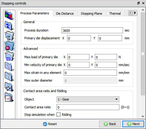
Stopping controls window

Under Process Conditions , Set the environment temperature to 850 C and change the convection coefficient to 0.1. This convection coefficient is similar to the convection coefficient of certain quench oil. (see Fig. 2DHTML1.24.) Click on to DB generation page..

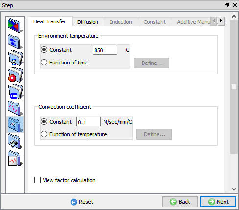
Process Conditions window

Generate Database

In Generate DB page. Click the button to have the program check to see if anything was missed in the problem setup. During the checking process, messages in the red color signify data that needs to be fixed before a simulation can be run (such as when you forget to define any material data).If there are no errors shown, then the database can be generated.

Click on button to generate the database (see Fig. 2DHTML1.25.). When the program is done writing the database, switch to tab to run simulation.

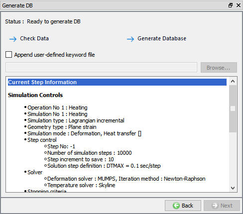
Generate DB window

Running a Simulation

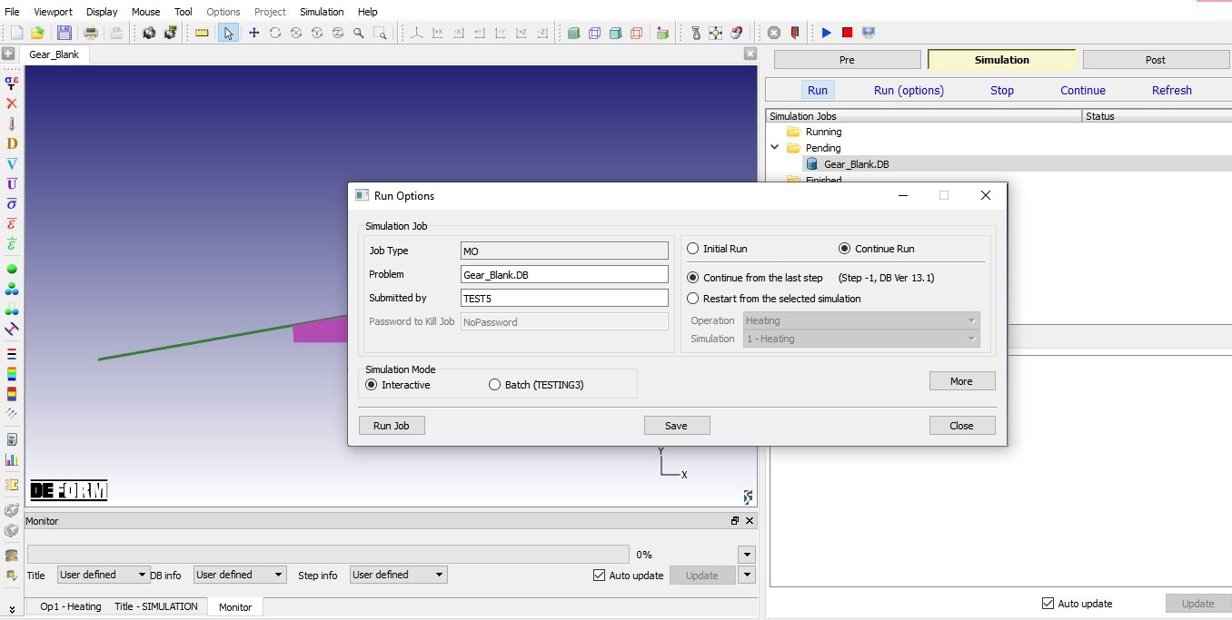
Click on the action label to open the Run Options dialog as shown in Fig. 2DHTML1.26. Use the default Continue Run option to select “Continue from the last step ” option and then select the Simulation mode as Interactive and click on button to run the simulation.

Run Simulation window

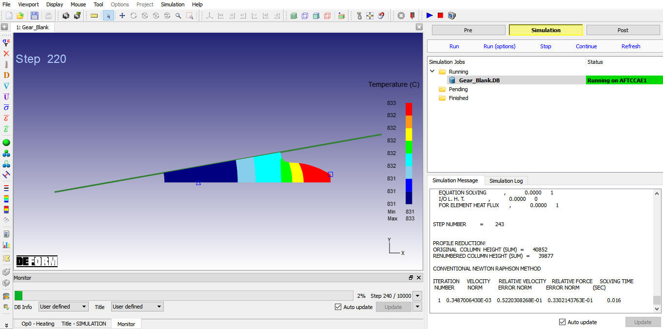
The progress of the simulation can be monitored as it is running by looking at the Simulation Message and process monitor in Simulation mode. Click the Simulation Message tab to view the Message file. the Message file will refresh every couple of seconds.

The Message file provides information about which simulation step the simulation is currently on and also gives information dealing with how well the simulation is running.(See Fig. 2DHTML1.27.)

Simulation Message

Post-Processing the Results

After simulation has been completed, switch to tab to view results, MO post processor will open.

The key state variable to investigate is the phase volume fraction. Click the State Variables button to open the state variable dialog. Open the variable Volume Fraction under the Microstructure tab. Select the Pearlite component and plot the variable as a shaded contour. The user should see the variable initially having a value of 1.0 (which means 100 % of the structure is composed of Pearlite) and eventually falling to 0.0 (which means 0 % of the material is composed of Pearlite). The user should plot the other volume fractions to determine which component the volume was converted to.(See Fig. 2DHTML1.28.). Click the StateVariables button and Plot Temperature (See Fig. 2DHTML1.29.)

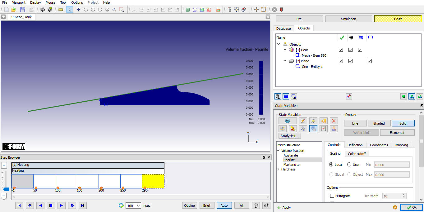
Volume fraction-Pearlite plot

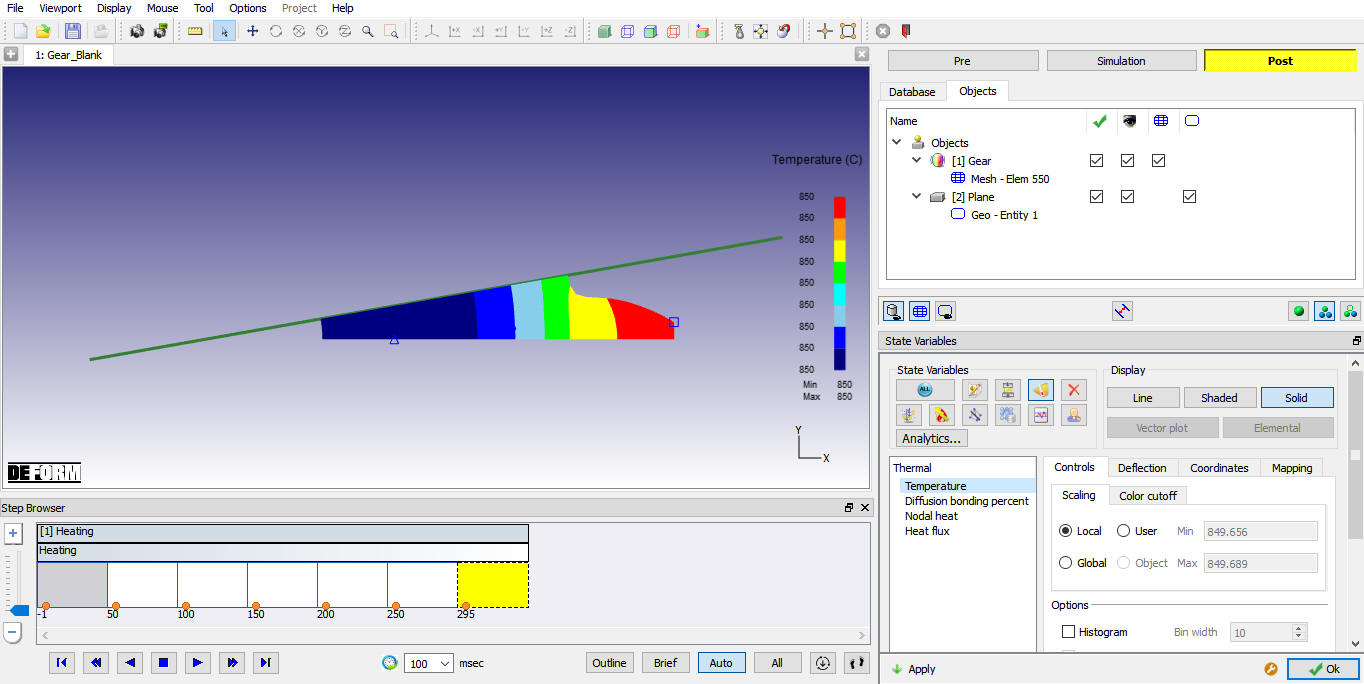
Temperature plot

In addition, user should look at the volume change of the object as a function of time. Click on the Summary icon to open the Summary dialog. plot the Volume. A plot of object volume as a function of time should appear as shown in Fig. 2DHTML1.30. Noted that without phase transformation, the object volume would have increased monotonically with temperature due to thermal expansion. With transformation, there is a dip in volume during transformation. This is because austenite is the FCC structure while Pearlite consists of ferrite (BCC structure) and cementite (orthorhombic structure). FCC is a closed packed structure and hence smaller in volume than either BCC or any orthorhombic structure, causing Pearlite austenite transformation to decrease the volume.

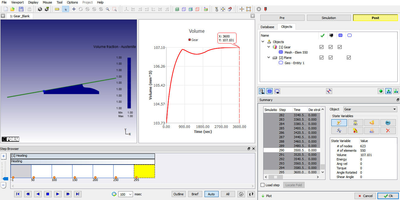
Summary window Volume plot

Exiting MO wizard

When you are finished, exit the MO Post-processor by clicking the close icon, a popup will appear to save the changes. Click for the popup and MO wizard will close.

(Or)

If User wants to continue the setup, can switch to pre mode directly and continue the setup by adding operation.