Flow Forming Lab

In this Lab we will be setting up simple Forward Flow forming process.

1.1. Creating a New Problem

1.2. Process Page

1.3. Simulation Setup

1.4. Objects selection

1.5. Workpiece

1.6. Mandrel

1.7. Head Stock

1.8. Tail Stock

1.9. Roll 1

1.10. Roll 2

1.11. Roll 3

1.12. Pass Table

1.13. Controls

1.14. Contact

1.15. Stopping controls

1.16. Simulation controls

1.17. Generate Database

1.18. Running Simulation

1.19. Post processing

Creating a New Problem

On a Windows machine , go to the button select DEFORM-v1x.xxx (.xxx indicates version number E.g. v14.0.2) and select DEFORM GUI Main vxx.xx from the menu. The DEFORM GUI Main window will appear.

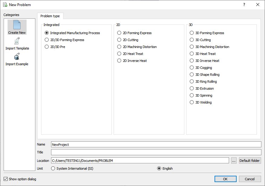
Create a new problem either by selecting File **New Problem** or by clicking the New Problem icon. The Problem Setup window will appear as shown in Fig. 3DFFL1.1. Select “ Integrated Manufacturing Process “ radio button and Unit system as “English “ using radio button. Define Problem Name as “Flowformlab “ and make sure the “Show option dialog” check box is turned on (if we do not turn on the “Show option dialog ” check box, then we will not get the New Project dialog in MO UI). Then click on button to open a new Problem using the Deform Integrated Manufacturing Process.

New Problem page

Multiple operation wizard will open with the New Project dialog, At this point user will be prompted to specify a project name (system will create a separate folder with this project name) and title for this session. In this session we will use ‘Flowformlab ’ as the project name. Click on to continue to open new project.

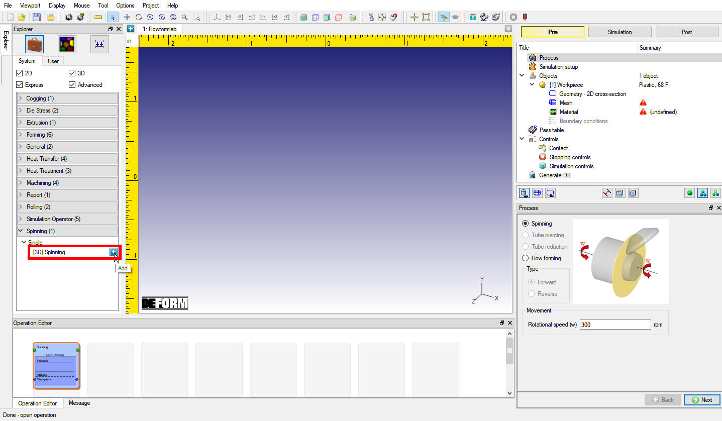
Add 3D Spinning operation from the Explorer Operations list. Add the operation by clicking on button available next to 3D Spinning or user can also add by drag and drop into the Operation Editor (see Fig. 3DFFL1.2.). When we add the Spinning operation, When we add the Spinning operation, If the current Screen upward direction is “Z “ direction then we will get below popup. Click “YES-Change “ in “Change screen upward axis” popup. Process settings Window will open by default. 3D Spinning operation can also be added in “New Project” dialog in MO.

Adding 3D Spinning operation

Process page

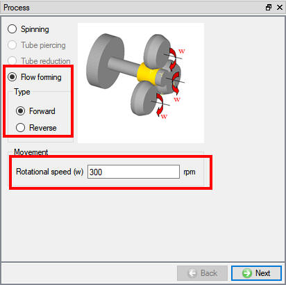
In Process page select “Flow forming “ and type of flow forming as “Forward “. Define Mandrel Rotationalspeed as 300 rpm, see Fig. 3DFFL1.3. This rotational speed will be applied to Head stock and Tail stock. Click on to Simulation setup page.

Process page

Simulation Setup

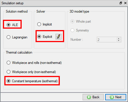
In Simulation Setup page select solution method as “ALE “ and solver type as “Explicit “. We will not be doing any thermal calculations in this lab hence select Thermal Calculation as “Constant temperature (isothermal) “ (see Fig. 3DFFL1.4.). Click to set Explicit solver controls as follows.

Simulation setup page

• Set Damping coefficient to 1. This dampens vibrations. A setting of 0-1 is conservative and 5-10 is more aggressive.

• Set Massscalingfactor to 200. This affects the time step, accuracy and runtime. A lower mass scaling factor results in a smaller time step and greater accuracy, but it requires a longer simulation time. This can be adjusted as needed, based on experience, application and goals.

• Set Cycle to 100. This controls the ratio of explicit solution cycles per step. The combination of this setting and the database step save increment can be used to adjust how often cycles are written to the database. A setting of 0 results in 1 cycle per step (1:1 ratio). A setting of 100 results in 100 cycles per step (100:1 ratio). Click on to close Explicit solvers settings page. Click on to Objects page.

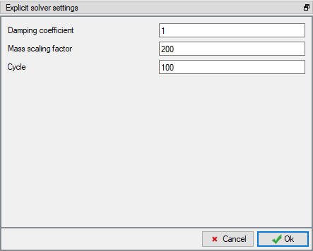
Explicit solvers settings

Objects selection

In the “Number of Objects ” page define number of rollers as 3 , In the table below Number of rolls definition user can define angle between rolls, for this lab we will use with default value of 120 ° for and . Check the Mandrel, Head stock and Tail stock check box (if not checked) (see Fig. 3DFFL1.6.) to use these objects in the setup. Tail stock is not used in reverse flow forming process and optional in forward flow forming. Click on to Workpiece General page.

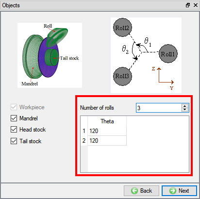
Object selection page

Workpiece

In the Workpiece object page keep the default values for name as workpiece and temperature 68°F. Change the Object type to “Elasto-plastic “ as shown in Fig. 3DFFL1.7., for explicit solver type simulation setups the workpiece must be Elasto-plastic object type. Click on to Geometry 2D cross- section page.

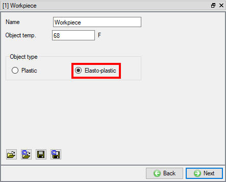
Workpiece page

Workpiece 2D cross section

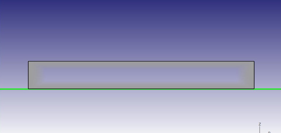
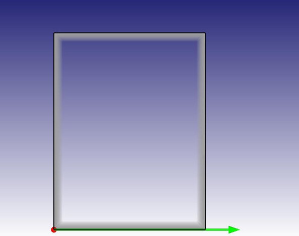
Import 2D geometry, “workpiece_lab.GEO ” from the 3D/LABS/Spinning folder. You can edit, check or save 2D geometry in this page as shown in Fig. 3DFFL1.8. Click on to Mesh page.

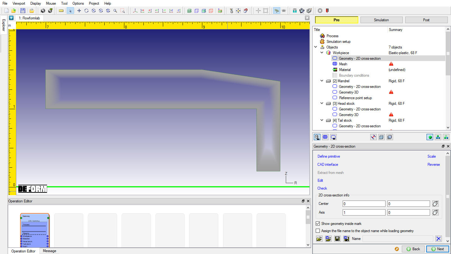
Workpiece Geometry 2D cross-section page

Workpiece Mesh

Define Number of elements for 2D cross section as 100 and click on . Define Number of revolved sections as 100 , pick “Uniform thickness of layers in hoop direction “ which is preferred for explicit solver and click on . Generated 2D and 3D mesh should look like as shown in Fig. 3DFFL1.9. and Fig. 3DFFL1.10. Click on to Material page.

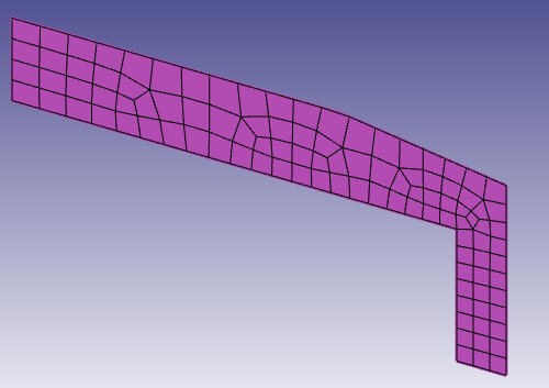
Generated 2D Mesh for Workpiece

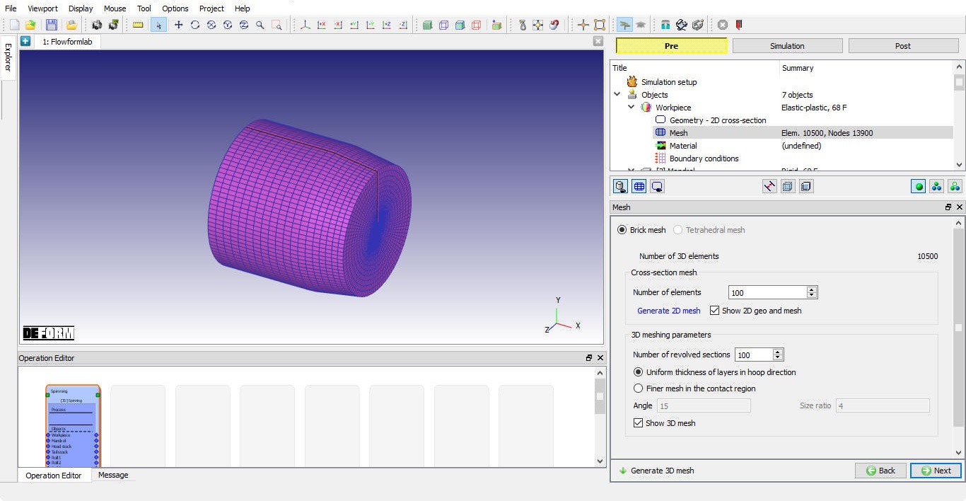
Generated 3D Mesh for Workpiece

Assign Material for Workpiece

In Material page, click on (Load material from library) icon and load the material Aluminum group material “AL-3003,COLD[70-250F(20-120C)] “ from material library window. Assign the “AL-3003,COLD[70-250F(20-120C)] “ material for Workpiece as shown in Fig. 3DFFL1.11. Click on until Mandrel page.

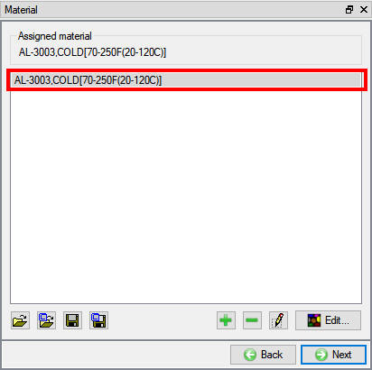
Workpiece Material page

Mandrel

In the Mandrel general page keep the default values for name as Mandrel and temperature as 68°F. Click on to Geometry 2D cross- section page.

Mandrel Geometry - 2D Cross-section

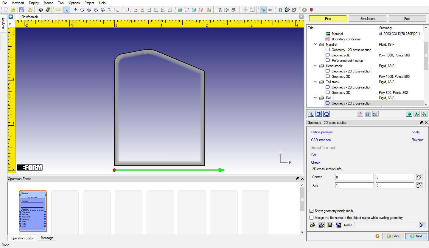
Import 2D geometry, “mandrel_lab.GEO ” from the 3D/LABS/Spinning folder. You can edit, check or save 2D geometry in this page as shown in Fig. 3DFFL1.12. Click on to Geometry - 3D page.

Mandrel Geometry - 2D Cross-section

Mandrel 3D Geometry

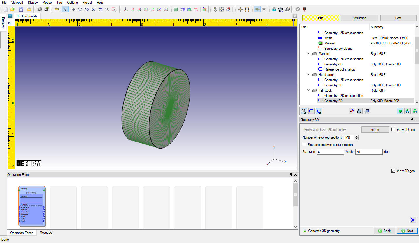
Using default “Number of revolved sections “ as 100 , generate 3D geometry by clicking on option (see Fig. 3DFFL1.13.). Fine Geometry at Contact region is not required for Explicit solver hence can be left as unchecked. Click on to Reference point setup page.

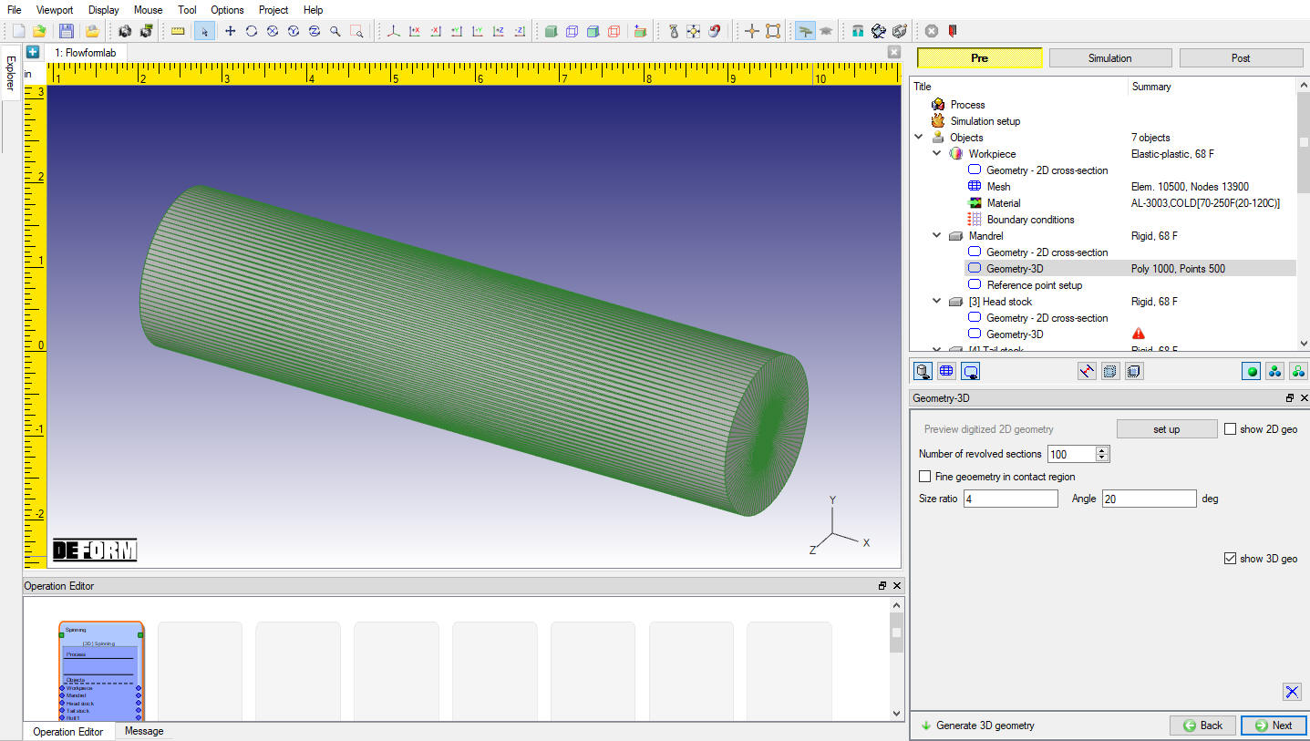
Mandrel Geometry-3D

Mandrel Reference Point setup

In this page we can define Reference point of Mandrel, we will use default value of D “1.99 “ as shown in Fig. 3DFFL1.14. “D ” is the distance between the Deform Origin and the origin of the Mandrel along X axis and will be used to position the mandrel. Click on to Head Stock page.

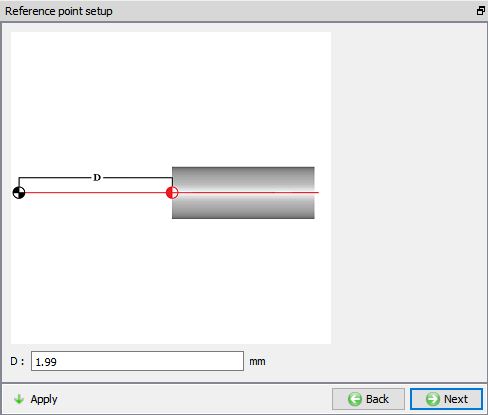
Mandrel Reference Point setup page

Head Stock

In the Head Stock general page keep the default values for name as Head stock and temperature as 68°F. Click on to Geometry 2D cross- section page.

Head Stock Geometry - 2D Cross-section

Import 2D geometry, “Headstock_lab.GEO ” from the 3D/LABS/Spinning folder. You can edit, check or save 2D geometry in this page as shown in Fig. 3DFFL1..15. Click on to Geometry - 3D page.

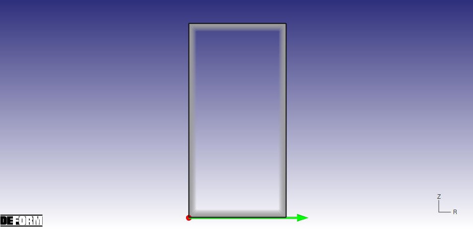
Head stock Geometry - 2D Cross-section

Head Stock 3D - Geometry

Using default “Number of revolved sections “ as 100 , generate 3D geometry by clicking on option (see Fig. 3DFFL1.16.). Click on to Tail stock page.

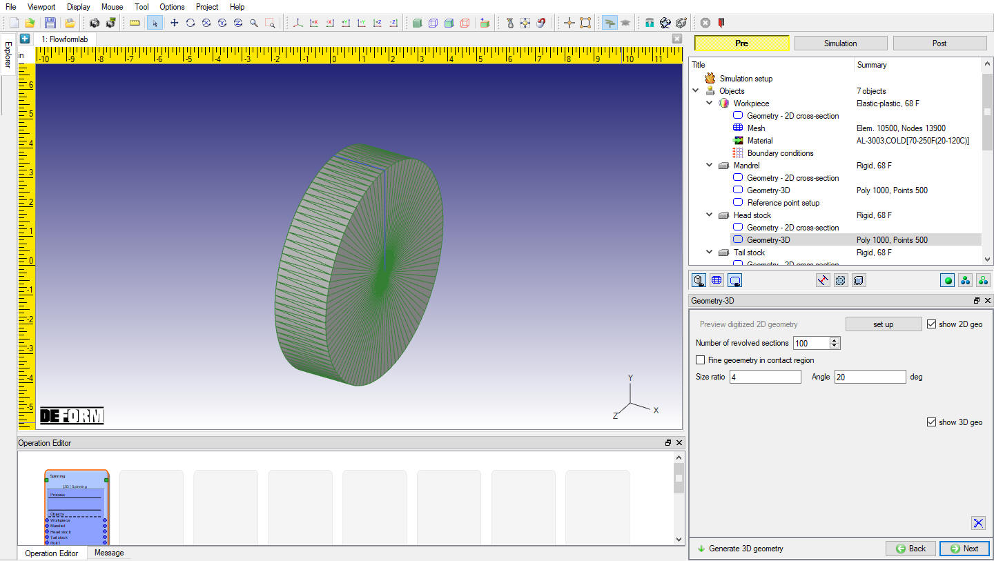
Head stock Geometry-3D page

Tail Stock

In the Tail Stock General page keep the default values for name as Tail stock and temperature as 68°F. Click on to Geometry 2D cross- section page.

Tail Stock Geometry - 2D Cross-section

Import 2D geometry, “tailstock_lab.GEO ” from the 3D/LABS/Spinning folder. You can edit, check or save 2D geometry in this page as shown in Fig. 3DFFL1.17. Click on to Geometry - 3D page.

Tail stock Geometry - 2D Cross-section

Tail Stock 3D - Geometry

Using default “Number of revolved sections “ as 100 , generate 3D geometry by clicking on option (see Fig. 3DFFL1.18.). Click on to Roll page.

Tail Stock Geometry-3D page

Roll 1

In the Roll 1 general page keep the default values for name as Roll 1 and temperature as 68°F. Click on to Geometry 2D cross- section page.

Roll 1 Geometry - 2D Cross-section

Import 2D geometry, “roller_lab.GEO ” from the 3D/LABS/Spinning folder. You can edit, check or save 2D geometry in this page as shown in Fig. 3DFFL1.19. Click on to Geometry - 3D page.

Roll 1 Geometry - 2D Cross-section

Roll 1 3D Geometry

Using default “Number of revolved sections “ as 100 , generate 3D geometry by clicking on option (see Fig. 3DFFL1.20.). Click on to orientation page.

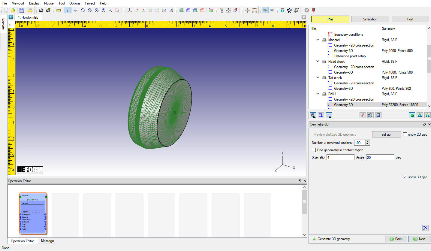
Roll 1 Geometry-3D page

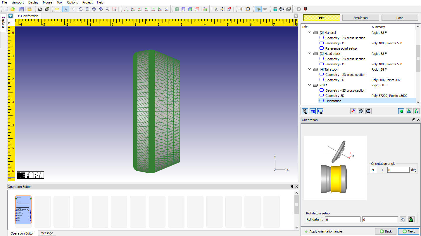
Roll 1 Orientation

In this page we can modify the orientation angle of Roll using Roll Orientation angle option and also the Roll datum point can be selected using roll datum setup options.

In this lab we are not changing the orientation angle and Roll datum point of Rolls, so click to Roll 2 page without any changes.

Roll1 Orientation page

Roll 2

In the Roll 2 general page keep the default values for name as Roll 2 and temperature as 68°F. Click on to Geometry 2D cross- section page.

Roll 2 Geometry - 2D Cross-section

Import 2D geometry, “roller_lab.GEO ” from the 3D/LABS/Spinning folder. You can edit, check or save 2D geometry in this page as shown in Fig. 3DFFL1.19. Click on to Geometry - 3D page.

Roll 2 3D - Geometry

Using default “Number of revolved sections” as 100, generate 3D geometry by clicking on option (see Fig. 3DFFL1.20.). Click on to orientation page.

Roll 2 Orientation

In this labwe are not changing the orientation angle and Roll datum point of Rolls, so click on to Roll 3 page without any changes.

Roll 3

In the Roll 3 general page keep the default values for name as Roll 3 and temperature as 68°F. Click on to Geometry 2D cross- section page.

Roll 3 Geometry - 2D Cross-section

Import 2D geometry, “roller_lab.GEO ” from the3D/LABS/Spinning folder. You can edit, check or save 2D geometry in this page as shown in Fig. 3DFFL1.19. Click on to Geometry - 3D page.

Roll 3 3D-Geometry

Using default “Number of revolved sections “ as 100 , generate 3D geometry by clicking on option (see Fig. 3DFFL1.20.). Click on to orientation page.

Roll 3 Orientation

In this lab we are not changing the orientation angle and Roll datum point of Rolls, click to pass table page.

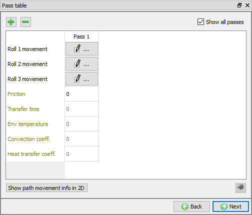
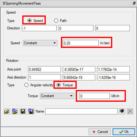
Pass Table

Here we will be defining Rolls Speed along the mandrel axis as 0.25 in/sec. For this lab we will be considering rolls to rotate based on free torque hence we will select Torque in Rotation tab and define its value as0 klb-in. So, click on Roll 1 button in Pass table and define speed as 0.25 in/sec and Torque as 0 klb-in as shown in Fig. 3DFFL1.23. and click on to close the movement page. Define the same movement data in Roll 2 and Roll 3 movement page by clicking on respective button. We will not define any other data from pass table as of now. Click on to Controls page.

Pass table page

Roll 1 Movement page

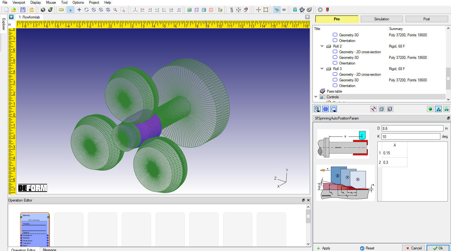
Controls

Click on “Automatic Positioning “, define the parameters

D=8.6 , Distance between head stock surface and the Roll Datum point

K=10 , orientation angle of the rolls with workpiece

A1=0.15 , A2=0.3 , Lateral distance between rolls along the mandrel axis

Click on to change the apply settings. It will position all 3 rollers and Workpiece and Tail stock in correct position as shown in Fig. 3DFFL1.24. Click on to close Automatic position page. Click on to Contact page.

Automatic position window

Contact

The Flowforming setup will assume a low shear friction for the mandrel and tailstock. This will be similar to cold forming where material is sliding along a die surface. A high shear friction, typical of rolling, will be assumed for the roller. Local contact searching is used to reduce contact search calculation time, which is useful with explicit simulations. For each object pair, friction windows must be defined over the area of the tool where contact may occur. Areas outside the window will not be considered for contact. The friction settings found on the friction window menu take precedence over the global settings. Friction windows must be set to follow moving tools, when applicable.

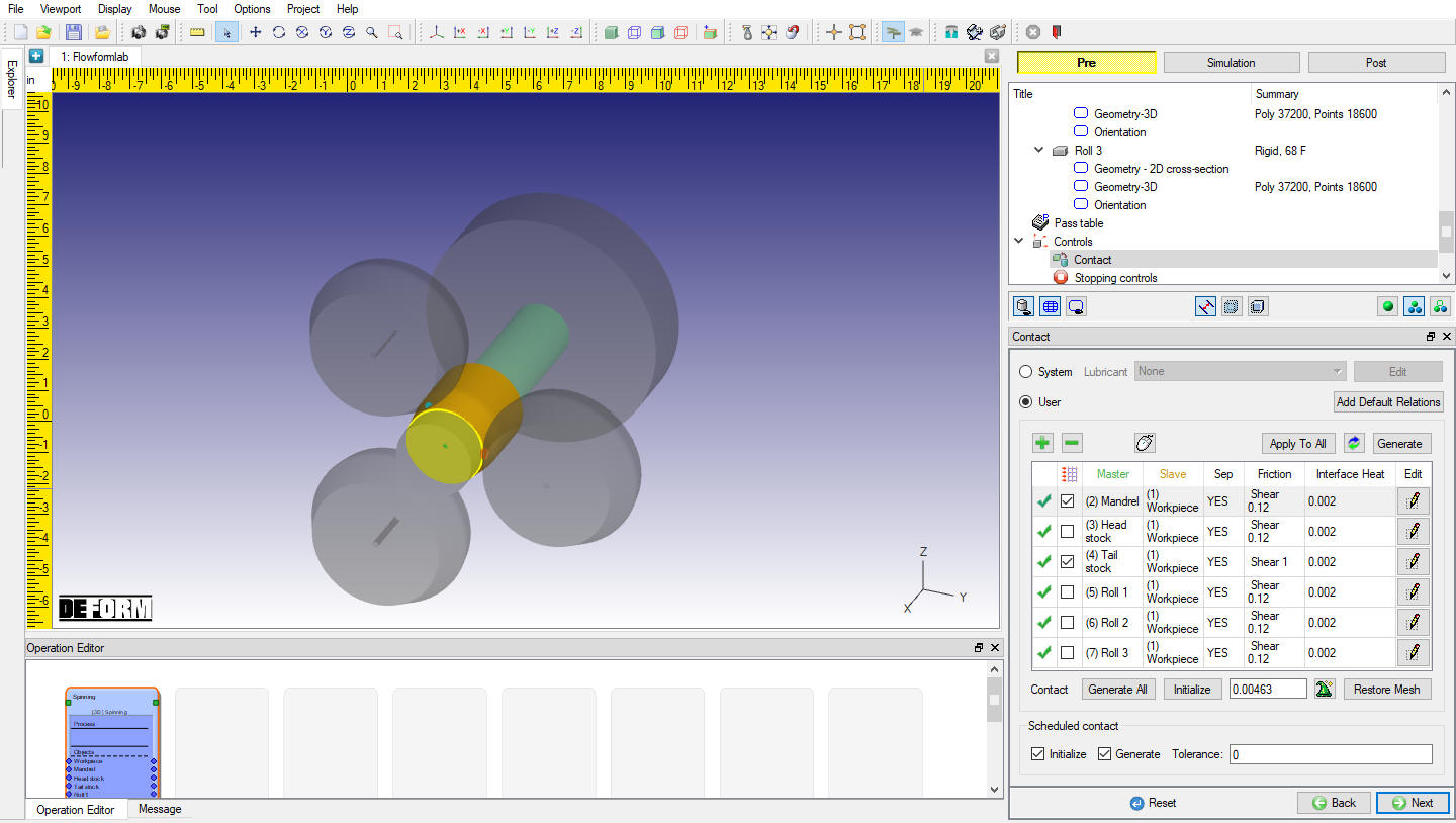
In Contact page, select “User “ type and click on button. In table, we will be observing default relations being added and sticking contact will be checked for Tail stock - Workpiece and Head stock - Workpiece relations. For this lab, we will turn on Mandrel - Workpiece sticking check box and turn off Head stock - Workpiece sticking check box and as shown in Fig. 3DFFL1.30.

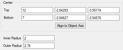
• Select theMandrel - Workpiece relation and . Define a Shear friction of 0.12. Switch to the Friction Window tab. Click the button to add a new window. Click on the Solid cylinder button on toolbar that is along the far-left side of the screen. Click anywhere on the model to place the window. Click the icon to define the window size as shown in the Fig. 3DFFL1.25., click . Select Shear friction and set a constant value of 0.12 and select “Mandrel “ as object to follow window, click .

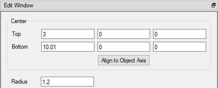
Mandrel - workpiece window definition

• Select the Head stock - Workpiece relation and . Define a Shear friction of 0.12 and click .

• Select the Tail stock - workpiece relation and . Define a Shear friction of 1. Switch to the Friction Window tab. Click the button to add a new window. Click on the Solid cylinder button on toolbar that is along the far-left side of the screen. Click anywhere on the model to place the window. Click the icon to define the window size as shown in the Fig. 3DFFL1.26., click . Select Shear friction and set a constant value of 1 and select “Tail stock” as object to follow window, click .

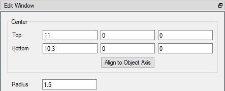
Tail stock - workpiece window definition

• Select the Roll 1 - Workpiece relation and . Define a Shear friction of0.12. Switch to the Friction Window tab. Click the button to add a new window. Click on the Hollow cylinder button on toolbar that is along the far-left side of the screen. Click anywhere on the model to place the window. Click the icon to define the window size as shown in the Fig. 3DFFL1.27., click . Select Shear friction and set a constant value of 0.12 and select “Roll 1” as object to follow window, click .

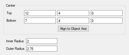
Roll 1 - Workpiece window definition

• Select the Roll 2 - Workpiece relation and . Define a Shearfriction of 0.12. Switch to the Friction Window tab. Click the button to add a new window. Click on the Hollow cylinder button on toolbar that is along the far-left side of the screen. Click anywhere on the model to place the window. Click the icon to define the window size as shown in the Fig. 3DFFL1.28., click . Select Shear friction and set a constant value of 0.12 and select “Roll 2” as object to follow window, click .

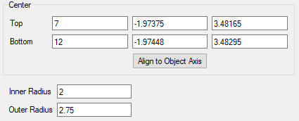
Roll 2 - Workpiece window definition

• Select the Roll 3 - Workpiece relation and . Define a Shear friction of 0.12. Switch to the Friction Window tab. Click the button to add a new window. Click on the Hollow cylinder button on toolbar that is along the far-left side of the screen. Click anywhere on the model to place the window. Click the icon to define the window size as shown in the Fig. 3DFFL1.29., click . Select Shear friction and set a constant value of 0.12 and select “Roll 3 “ as object to follow window, click .

Roll 3 - Workpiece window definition

Click on button to calculate the default tolerance value and Generate contact by clicking on button and also select Yes in “STICKING CONDITION “ popup. Generated contact will look like as shown in Fig. 3DFFL1.30. Click on to Stopping controls page.

Contact Page

Stopping controls

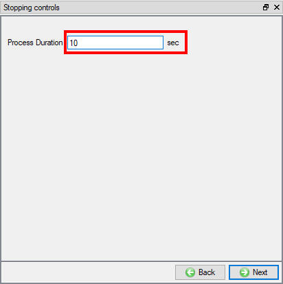
Define Process Duration as 10 sec in Stopping controls page (see Fig. 3DFFL1.31.). Click on to Simulation controls page.

Stopping Criteria page

Simulation controls

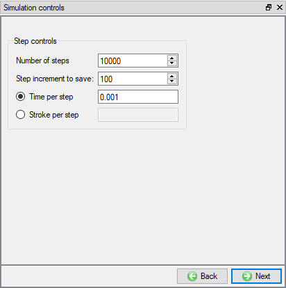
Enter Number of steps as 10000 , Step increment to save as 100 and Time per step as 0.001 in Simulation controls page (see Fig. 3DFFL1.32.). Click on to Generate DB page.

Simulation Controls page

Generate Database

In Generate DB page, click on the button to generate the database. Observe the message in Message tab informing database generation status.

Running Simulation

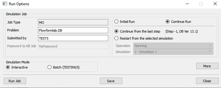
Once the database has been generated, switch to the Simulation mode by selecting the button above the object tree. Click on the action label to open the Run Options dialog as shown in Fig. 3DFFL1.33.. Use the default Continue Run option to select “Continue from the last step ” option and then select the Simulation mode as Interactive and click on button to run the simulation.

Run Simulation Window

Monitor the progress of the simulation by looking at the Simulation Message and Simulation Log tab, making sure that the option is checked. User can view the Flow Forming process as the simulation proceeds to the specified stopping criteria from Simulation graphics.

Post processing

When the simulation is completed, review the results by switching to Post mode using the button above the Simulation tool bar.

Play through the steps of the simulation and look how the Workpiece part is formed in Flow forming process.

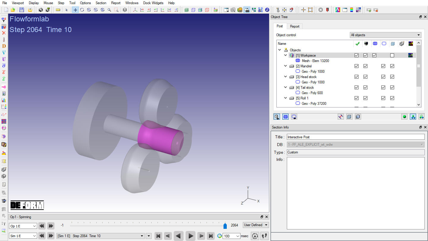
Flow forming operation last step

Plot Effective Strain State variable and observe the Strain distribution (see Fig. 3DFFL1.35.).

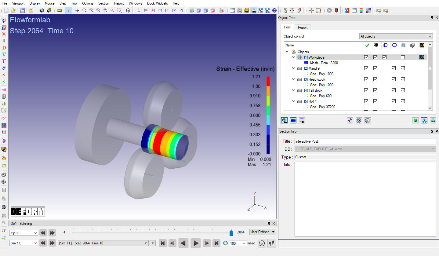
Effective Strain distribution at last step