Lab 04 Heat Transfer
4.1. Creating a New problem
4.2. Adding Heat Transfer operation
4.3. Changing operation Name
4.4. Heating in Furnace
4.5. Heating in Furnace Process
4.6. Furnace Heat Condition
4.7. Workpiece Setup
4.8. Heating Furnace Step controls
4.9. DB Generation for Heating Furnace
4.10. Air Cool operation
4.11. Air cool operation Process page
4.12. Step Controls For Air cooling
4.13. DB Generation For Air Cooling
4.14. Starting the Simulation
4.15. Post-Processing the Results
In this lab we will setup two operation:
Operation 1 - Heating in Furnace : In this operation, we are heating the billet in a furnace for 1 hour at 1800°F temperature environment.
Operation 2 - Air cool operation: In this operation, we are cooling the billet in room temperature for 60 seconds.
Creating a New problem
On a Windows machine , go to the ![]() button select DEFORM-v1x.xxx (.xxx indicates version number E.g. v14.0.2) and select DEFORM GUI Main vxx.xx from the menu. The DEFORM GUI Main window will appear. as shown below Fig. L4.1.
button select DEFORM-v1x.xxx (.xxx indicates version number E.g. v14.0.2) and select DEFORM GUI Main vxx.xx from the menu. The DEFORM GUI Main window will appear. as shown below Fig. L4.1.
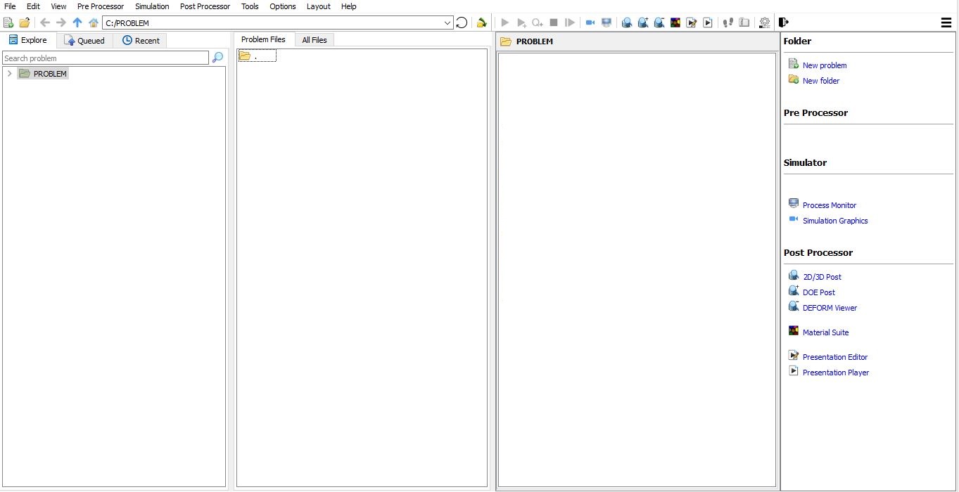
DEFORM-2D/3D GUI main window
Create a new problem either by selecting File![]() New Problem or by clicking the New Problem
New Problem or by clicking the New Problem ![]() icon. The Problem Setup window will appear as shown in Fig. L4.2. Select “ Integrated Manufacturing Process “ radio button and unit system as “English “ using radio button. Define Problem Name as “Heat_Transfer “ and make sure the “Show option dialog ” check box is turned on (if we do not turn on the “Show option dialog” check box, then we will not get the New Project dialog). Then click on
icon. The Problem Setup window will appear as shown in Fig. L4.2. Select “ Integrated Manufacturing Process “ radio button and unit system as “English “ using radio button. Define Problem Name as “Heat_Transfer “ and make sure the “Show option dialog ” check box is turned on (if we do not turn on the “Show option dialog” check box, then we will not get the New Project dialog). Then click on ![]() button to open a new problem using the Deform Integrated Manufacturing Process.
button to open a new problem using the Deform Integrated Manufacturing Process.
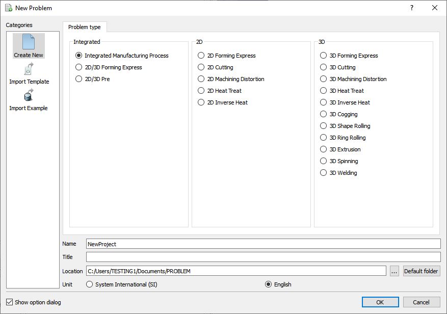
Problem type selection window
Multiple operation wizard will open with the New Project dialog (See Fig. L4.3.), at this point user will be prompted to specify a project name (system will create a separate folder with this project name) and title for this session. In this session we use ‘Heat_Transfer ’ as the project name. Select the Firstoperation as 2D Heat transfer operation and check the checkbox to add Heat transfer operation as first operation. Click on ![]() to continue to open the operation.
to continue to open the operation.
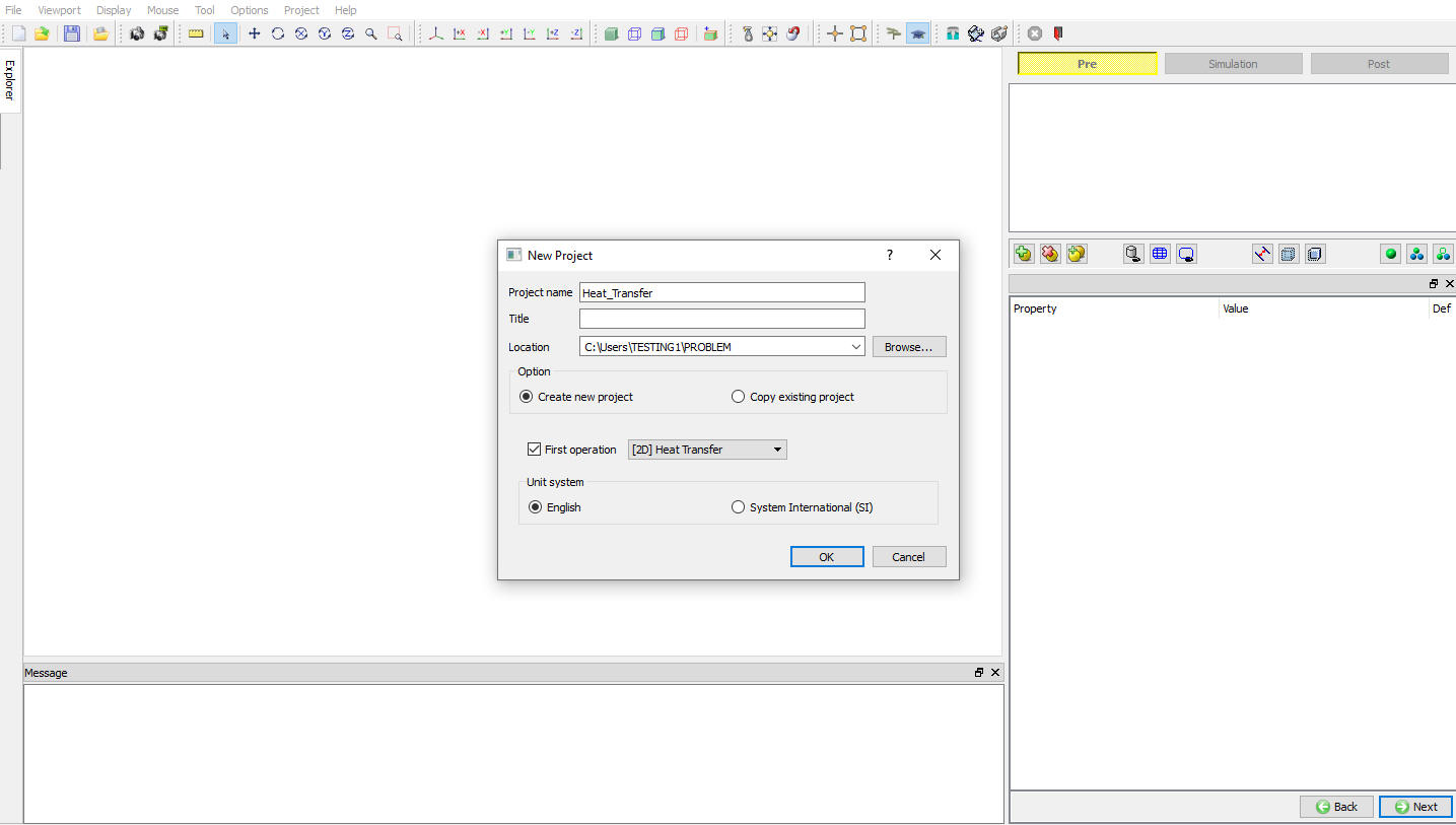
MO New project settings window
Adding Heat transfer operation
Multiple Operation wizard will opens the 2D heat transfer operation with new project called Heat_Transfer (See Fig. L4.4.). Add another 2D Heat Transfer operation as second operation from operation list in Explorer. Operation can be add by clicking on ![]() button next to 2D Heat Transfer operation or user can also add the operations by dragging and dropping the operation into Operation Editor region.
button next to 2D Heat Transfer operation or user can also add the operations by dragging and dropping the operation into Operation Editor region.
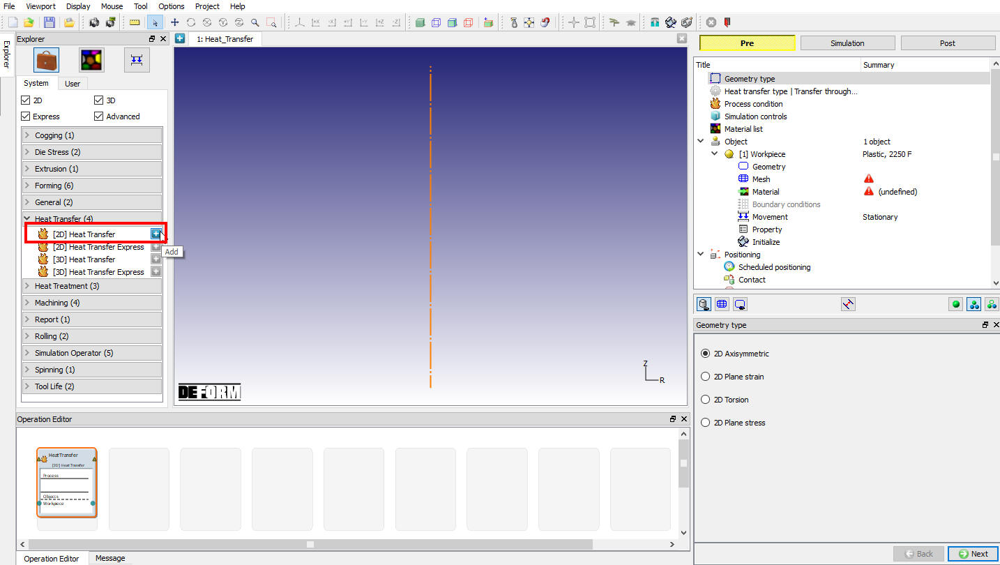
MO heat transfer project with 2d Heat Transfer operation
Changing operation Name
To change the operation name, double click on Heat Transfer field on 2D Heat transfer operation list in Operation editor, change the operation name to “Heating in Furnace “ and press Enter in Keyboard. repeat the same sequence to change the second Heat transfer operation name to “ Air cool “ , See Fig. L4.5. and Fig. L4.6.
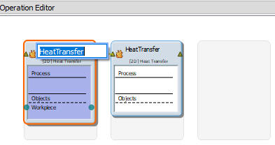
Changing Operation name from Operation Editor
After changing the operation name
Heating in Furnace
In this operation we are heating the billet at Room temperature in Heating furnace at 1800°F for 3600 seconds until it reaches steady state.
Heating in Furnace Process
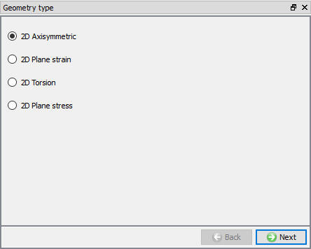
Highlight the first 2D Heat Transfer operation, in geometry type page select 2D Axisymmetric geometry type (See Fig. L4.7.). Click on ![]() button.
button.
Geometry type selection page
In Heat transfer type page, select Heat in furnace Heat transfer type as shown in Fig. L4.8.). Click on ![]() button.
button.

Heat Transfer type selection
Furnace Process condition
In Process Condition page, Change the Environment temperature to 1800 °F and use default process time as 3600 sec and use default Convective coefficient value in this lab. (see Fig. L4.9.) Then click on ![]() button. In simulation control select default setting and click on
button. In simulation control select default setting and click on ![]() button until Workpiece page.
button until Workpiece page.

Process condition page
Workpiece Setup
Change the Object Name to “ Billet “ and select object type as **(see Fig. L4.10.). At the start of the simulation, the billet will be going into the furnace, so the Temperature should be defined as room temperature, or 68°F. Click on ![]() button.
button.

Workpiece object window
Creating geometry
In Geometry page click on ![]() , enter the following XYR coordinates value in the Table 1. (See Fig. L4.11.) and click on
, enter the following XYR coordinates value in the Table 1. (See Fig. L4.11.) and click on ![]() button,
button,
| X | Y | R |
|---|---|---|
| 0 | 0 | 0 |
| 1.5 | 0 | 0.12 |
| 1.5 | 4 | 0.12 |
| 0 | 4 | 0 |
Geometry XYR coordinates value
Then click on ![]() button, Use the default checking parameters and click
button, Use the default checking parameters and click ![]() . A message saying, “Geometry is legal “ will appear. Then click on
. A message saying, “Geometry is legal “ will appear. Then click on ![]() and click on
and click on ![]() button.
button.

Workpiece Edit geometry page
Generating mesh
Use the default system mesh settings and click on ![]() . A mesh with approximately 1000 elements will be generated. Click on
. A mesh with approximately 1000 elements will be generated. Click on ![]() button.
button.
Assign Billet Material
In Material list window, load the material AISI-1025[1800-2200F(1000-1200C)] from DEFORM Material library, from Steel category using ![]() (Load material data from library) option. Then click on
(Load material data from library) option. Then click on ![]() , under Thermal tab of the material data, the
, under Thermal tab of the material data, the ![]() icon can be used for view the Heat capacity and thermal conductivity data. AISI-1025 has been loaded into the problem and it is automatically assigned to the Billet. Click on
icon can be used for view the Heat capacity and thermal conductivity data. AISI-1025 has been loaded into the problem and it is automatically assigned to the Billet. Click on ![]() button.
button.
Edit material window
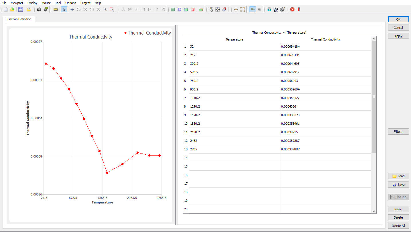
Thermal Conductivity material data

Heat Capacity material data
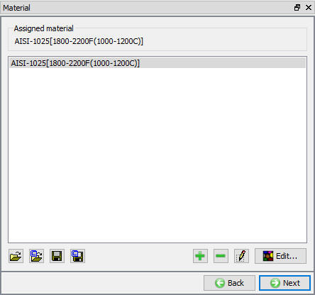
Object Material window
Defining Billet Heat Transfer Boundary Conditions
In BCC page, check the default assigned Heat exchange with Environment BCC to the entire outer surface of the Billet (which does not include the centerline since these nodes are inside the object) default BCC are assigned automatically due to selection of problem type as axisymmetric (See Fig. L4.16.). Then click on ![]() button until Step page.
button until Step page.
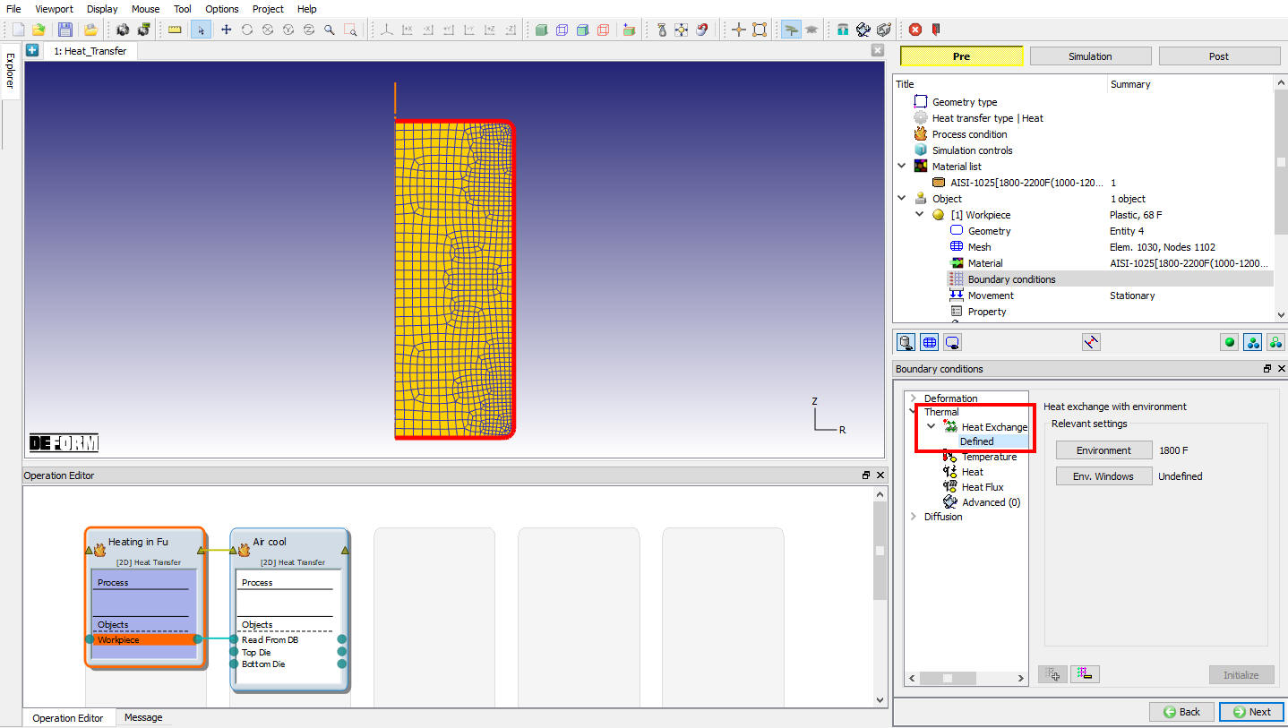
Billet BCC window
Heating Furnace Step controls
In Step page, change the Number of Steps to 240 , set increment to save as 10 and Solution step definition Time as 15 sec (See Fig. L4.17.), then click on ![]() button.
button.
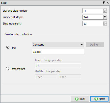
Step controls page
DB Generation for Heating Furnace
Once the operation has been completely set up, the last step is to generate a database file. The FEM engine (the part of DEFORM® that calculates the solution) uses a database file to store the finite element solutions for the problem. When you generate a database in the DEFORM MO Pre-processor, all of the information defined in the Pre-processor (such as the material properties, movement controls, object geometries, etc.) is transferred to the database file.
In Generate DB page. Click the ![]() button to have the program check to see if anything was missed in the problem setup. During the checking process:
button to have the program check to see if anything was missed in the problem setup. During the checking process:
Messages in the red color signify data that needs to be fixed before a simulation can be run (such as when you forget to define any material data).
Click on![]() button to generate the database. When the program is done writing the database, click on
button to generate the database. When the program is done writing the database, click on ![]() button to go to next operation.
button to go to next operation.
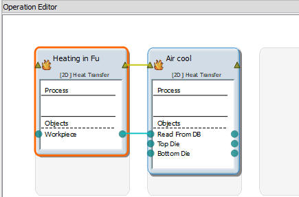
Air cool operation
In this operation we are cooling the billet in Room temperature for 60 seconds and the billet object is read from DB.
Air cool operation process page
In Process page, select Heat transfer type as Transfer through air. Click on ![]() button.
button.
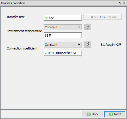
Change the Transfer time to 60 second, and use default Environment Temperature (68°F) and use default convective coefficient value as shown in Fig. L4.18. Click on ![]() until Object page. If Top die and Bottom Die objects are added in object list, then delete Object 2 and Object 3 using
until Object page. If Top die and Bottom Die objects are added in object list, then delete Object 2 and Object 3 using ![]() option. Click on
option. Click on ![]() until are Step page.
until are Step page.
Process condition window
Step Controls For Air cooling
In Steps page, change the Number of Steps to 60 , set increment to save as 4 and Solution step definition Time as 1 sec/step (See Fig. L4.19.), then click on ![]() button.
button.

Step controls page
DB Generation For Air Cooling
In Generate DB page see the status, if we are seeing status as “Input error” check the missing data and complete the setup. Save the project and switch to ![]() tab to run simulation.
tab to run simulation.
Starting the Simulation
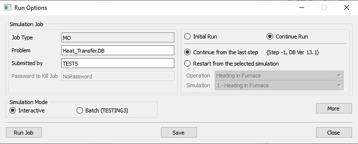
Click on ![]() under the simulation tab (See Fig. L4.20.), as we click on the Run option, Run simulation dialog will open (See Fig. L4.21.), Use the default Continue Run option to select “Continue from the last step ” option and then select the Simulation mode as Interactive and click on
under the simulation tab (See Fig. L4.20.), as we click on the Run option, Run simulation dialog will open (See Fig. L4.21.), Use the default Continue Run option to select “Continue from the last step ” option and then select the Simulation mode as Interactive and click on ![]() button to run the simulation.
button to run the simulation.

Simulation Options
Run Simulation window
The progress of the simulation can be monitored as it is running by looking at the Simulation Message and Simulation Graphics in Simulation mode. Click the Simulation Message tab to view the Message file. As long as the ![]() option is checked, which is the default setting, the Message file will refresh every couple of seconds.
option is checked, which is the default setting, the Message file will refresh every couple of seconds.
The Message file provides information about which simulation step the simulation is currently on and also gives information dealing with how well the simulation is running.
When the simulation has finished, the following message will be added to the end of the LOG file file: “MULTIPLE OPERATION COMPLETED.”
Post-Processing the Results
After simulation has been completed, switch to tab, MO post processor will open.
State variable Plot
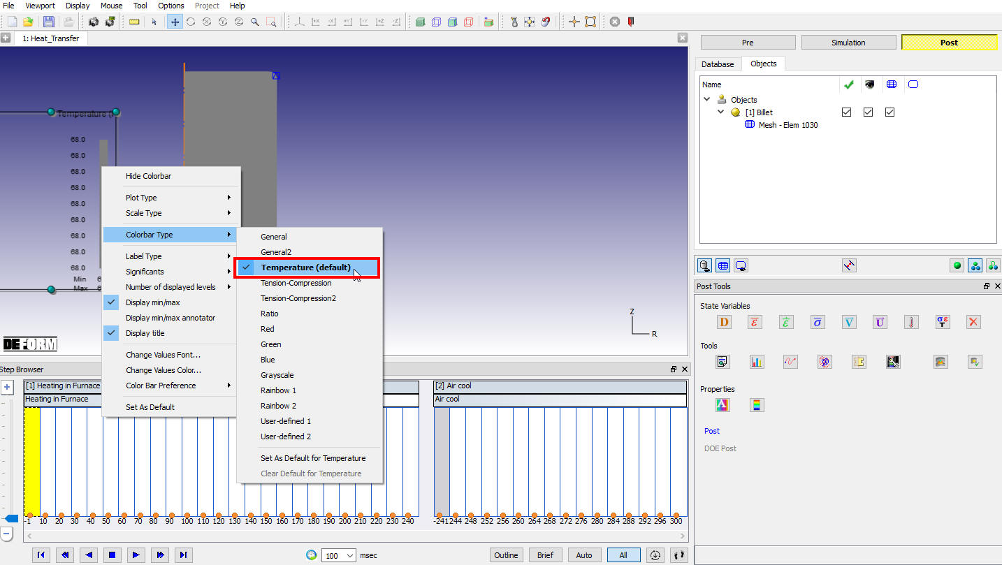
Click the ![]() icon and select Temperature as the variable. Right-click on the Color Bar in the DISPLAY window and select Temperature as the ColorBar Type. This provides a more intuitive color scheme when viewing temperatures (See Fig. L4.22.).
icon and select Temperature as the variable. Right-click on the Color Bar in the DISPLAY window and select Temperature as the ColorBar Type. This provides a more intuitive color scheme when viewing temperatures (See Fig. L4.22.).
Play through the steps and observe how the billet heats up in Heating operation and how it cools in Air cool operation (See Fig. L4.23.).
Plotting Temperature state variable with Temperature type Colorbar type
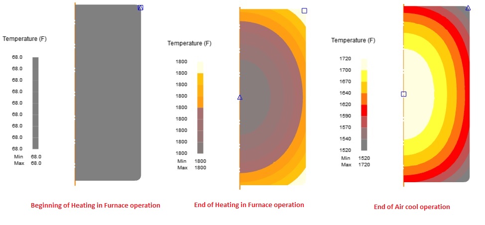
Temperature plot for Heat Transfer lab operations
Summary
The Summary button can be used to plot the minimum and maximum state variable graph. Click ![]() to open the SUMMARY window. To better understand how the billet heated up and cooling in this lab, select the Thermal tab and then click
to open the SUMMARY window. To better understand how the billet heated up and cooling in this lab, select the Thermal tab and then click![]() to Temperature (See Fig. L4.24.).
to Temperature (See Fig. L4.24.).
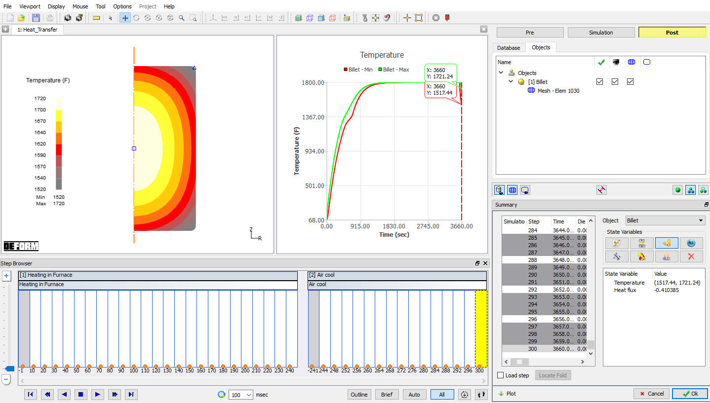
Temperature Summary plot
Point tracking
Temperatures at specific locations in the billet can be tracked using point tracking option.
Click the ![]() icon to open the POINT TRACKING window. Track the temperatures at three points halfway up the billet, at approximately the locations shown below Fig. L4.25. and Fig. L4.26.
icon to open the POINT TRACKING window. Track the temperatures at three points halfway up the billet, at approximately the locations shown below Fig. L4.25. and Fig. L4.26.

Selecting points for Point tracking
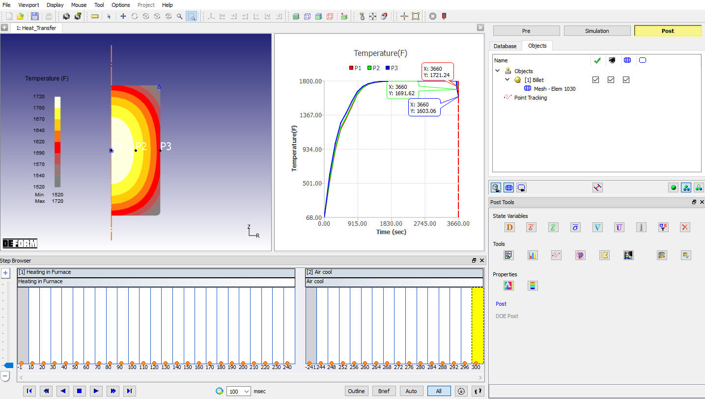
Temperature plot at selected region using point-tracking option
We would like to zoom in on the steps at the end of the simulation when the air cool takes place. Right click on Graph in display window and select set graph properties option in list, change the range of both the X-Axis and the Y-Axis to the values shown below Fig. L4.27. and click on ![]() .
.
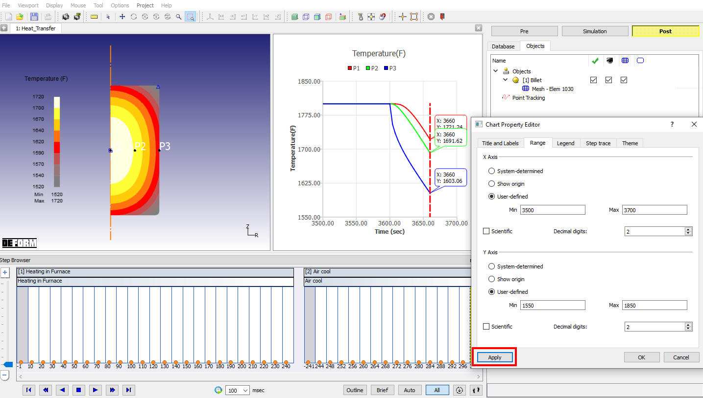
Graph Properties window
After these changes are made, it is much easier to see that the point on the OD of the billet (Point 3) cooled much faster than the point near the center (Point 1).
Related Topics:
35.1. 2D Heat Transfer Operation