Lab 25 Stub Shaft Labs
25.1. Stub Shaft Lab in 2D MO Forming
25.2. Tool Stress Analysis
25.3. Adding a Shrink ring to the Die
25.4. Simulating Thermal Effects
25.5. Warm Stub shaft with Mechanical press movement
25.6. Warm Stub shaft with Hydraulic press movement
25.7. Warm Stub shaft with Screw press movement
25.8. Warm Stub shaft with Hammer movement
Stub Shaft Lab in 2D MO Forming
In this lab we will setup 2 operations :
Operation1: Cone Operation.
Operation2: Head operation.
Operation1: Cone Operation
Create New Problem
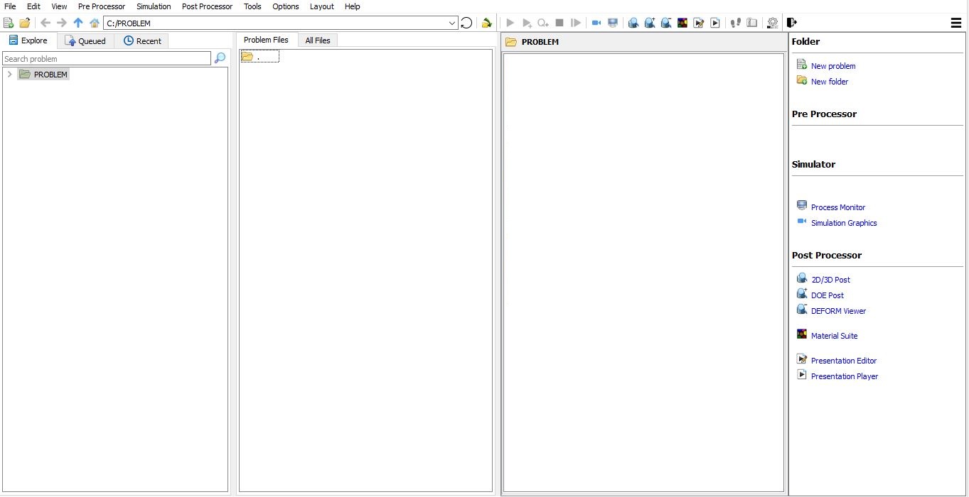
On a Windows machine , go to the ![]() button select DEFORM-v1x.xxx (.xxx indicates version number E.g. v14.0.2) and select DEFORM GUI Main vxx.xx from the menu. The DEFORM GUI Main window will appear as shown below Fig. L25.1.).
button select DEFORM-v1x.xxx (.xxx indicates version number E.g. v14.0.2) and select DEFORM GUI Main vxx.xx from the menu. The DEFORM GUI Main window will appear as shown below Fig. L25.1.).
DEFORM GUI Main
Create a new problem either by selecting File![]() New Problem or by clicking the New Problem
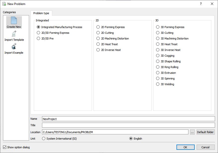
New Problem or by clicking the New Problem ![]() icon. The Problem Setup window will appear as shown in Fig. L25.2. Select “ Integrated Manufacturing Process “ radio button and unit system as “English “ using radio button. Define Problem Name as “Stub_Shaft “ and make sure the “Show option dialog ” check box is turned on (if we do not turn on the “Show option dialog” check box, then we will not get the New Project dialog). Then click on
icon. The Problem Setup window will appear as shown in Fig. L25.2. Select “ Integrated Manufacturing Process “ radio button and unit system as “English “ using radio button. Define Problem Name as “Stub_Shaft “ and make sure the “Show option dialog ” check box is turned on (if we do not turn on the “Show option dialog” check box, then we will not get the New Project dialog). Then click on ![]() button to open a new problem using the Deform Integrated Manufacturing Process.
button to open a new problem using the Deform Integrated Manufacturing Process.
Problem type selection window
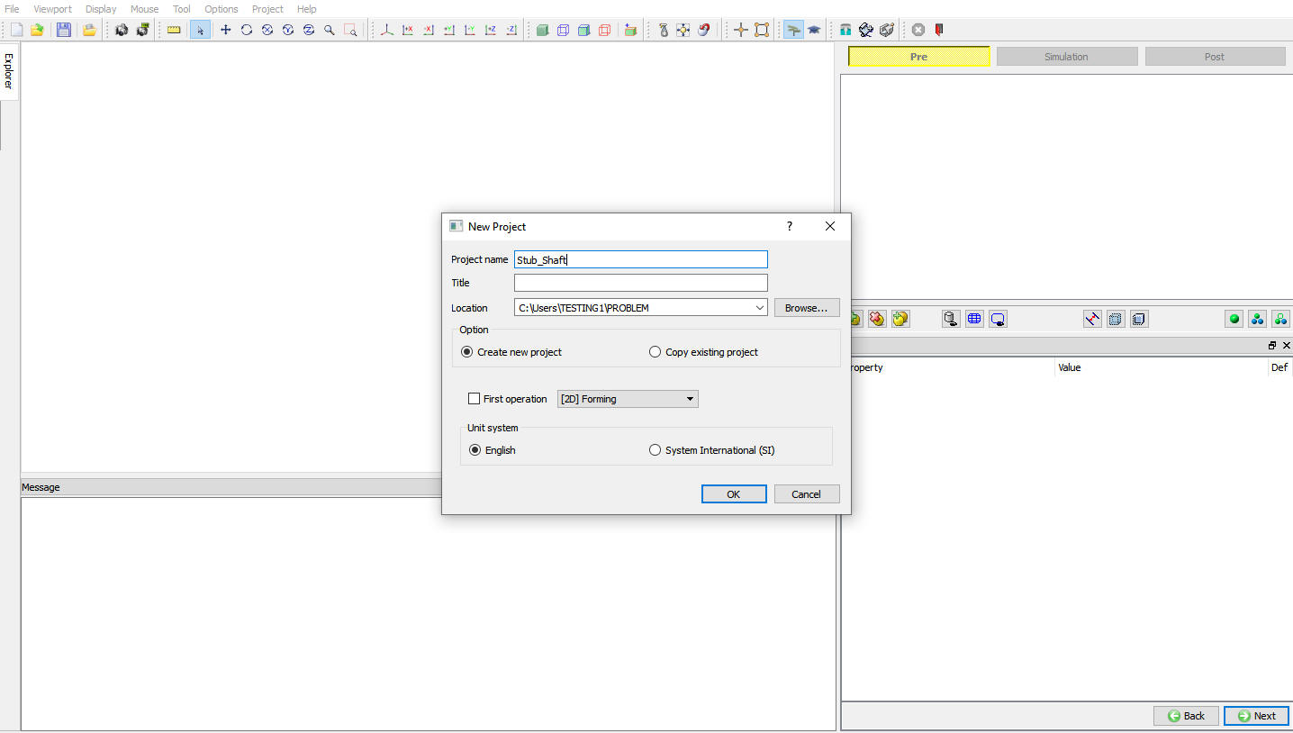
Multiple operation wizard will open with the New Project dialog (see Fig. L25.3.), at this point user will be prompted to specify a project name (system will create a separate folder with this project name) and title for this session. In this session we use ‘Stub_Shaft ’ as the project name. Click on ![]() to continue to open the operation.
to continue to open the operation.
MO wizard New Project
Adding 2D Forming operations
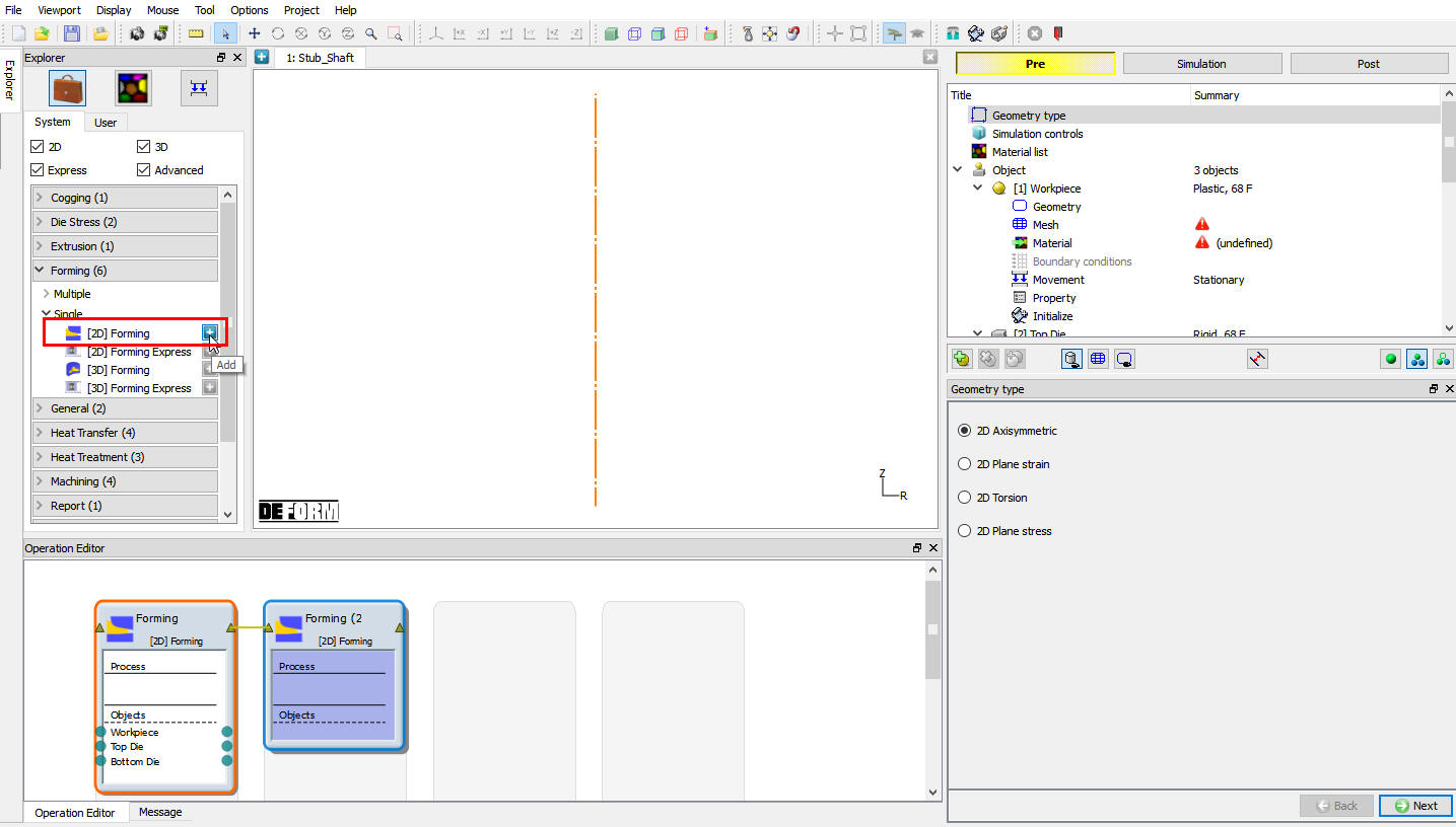
Multiple Operation wizard will opens with new project called Stub_Shaft to setup the problem. Add two2D Forming operations from Operations list in Explorer. Operation can be add by clicking on ![]() button next to 2D Forming operation (see Fig. L25.4.) or user can also add the operation by dragging and dropping the operation into Operation Editor region.
button next to 2D Forming operation (see Fig. L25.4.) or user can also add the operation by dragging and dropping the operation into Operation Editor region.
Added 2D Forming operation into Operation Editor
Geometry Type
In this lab we will be using Axisymmetric geometries, so select 2DAxisymmetric radio button from geometry type page as shown in Fig. L25.5. and click on ![]() .
.
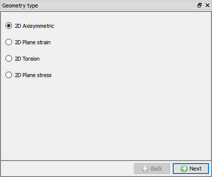
Axisymmetric Geometry type selection
Simulation Controls
In this lab we will be showing how to setup simple Isothermal problem. So in Simulation controls uncheck the Heattransfermode check box (see Fig. L25.6.). Then click on ![]() .
.
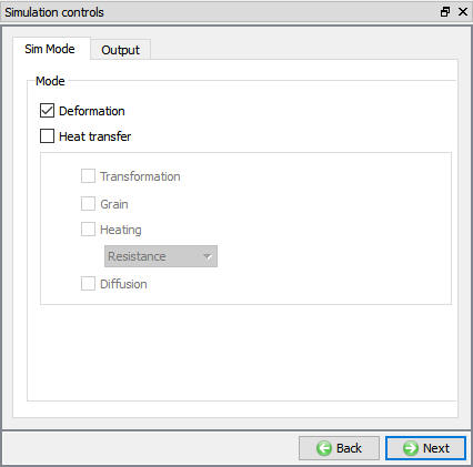
Simulation control window
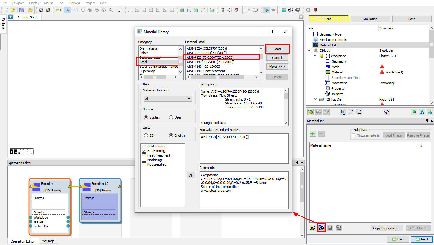
Assigning Material for Workpiece
In Material list window, Load the material ‘AISI-4120 ‘ from DEFORM Material library, Steel category using ![]() (Load material data from library) option. This can be done as shown in below by clicking
(Load material data from library) option. This can be done as shown in below by clicking ![]() button as shown in Fig. L25.7. Click on
button as shown in Fig. L25.7. Click on ![]() until Object page.
until Object page.
Material List window
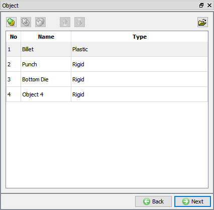
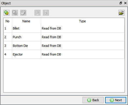
Adding objects
For this operation we required four objects, hence in Object window add four objects by clicking on ![]() button (see Fig. L25.8.) and click on
button (see Fig. L25.8.) and click on ![]() .
.
Adding Object Window
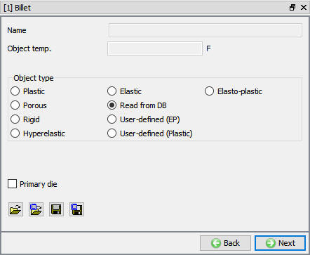
Workpiece
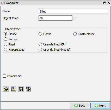
In Workpiece window, change the object Name to Billet and select object type as Plastic as shown in Fig. L25.9. Click on ![]() .
.
Billet object Window
Billet Geometry
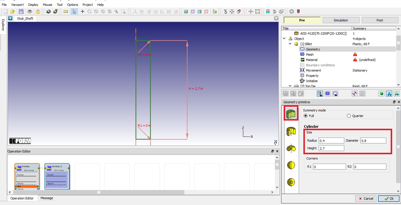
In the Geometry page, select ![]() and define a cylinder that has a radius of 0.4 ” and a height of 2.7 ” (see Fig. L25.10.). Click on
and define a cylinder that has a radius of 0.4 ” and a height of 2.7 ” (see Fig. L25.10.). Click on ![]() button. Check geometry and click on
button. Check geometry and click on ![]() .
.
Defining the Geometry
Mesh generation
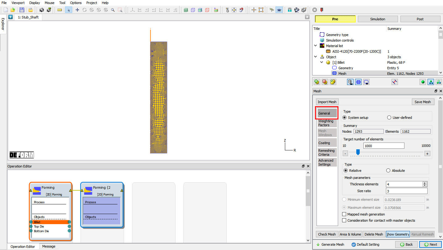
Switch to expert mode by clicking on ![]() , the default settings are adequate for generating a mesh. Click on
, the default settings are adequate for generating a mesh. Click on ![]() to generate the Mesh (see Fig. L25.11.).
to generate the Mesh (see Fig. L25.11.).
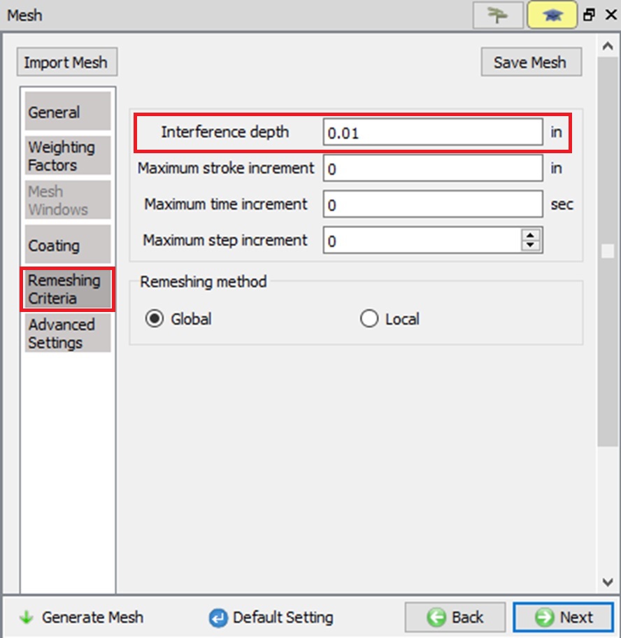
Measure one of the smaller elements in the workpiece – they are in the range of 0.020”. Click the Remesh criteria tab and set the Interference Depth to ½ of this value, or 0.01 ” This setting prevents excessive overlap between the tools and the workpiece as material flows around corners (See Fig. L25.12.). Click on ![]() .
.
Billet Mesh window
Defining Remeshing Criteria
Assigning Billet Material
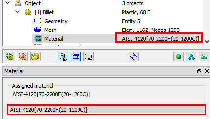
To assign material for workpiece select the material AISI-4120 from material window. This can be done as shown in below Fig. L25.13. Click on ![]() .
.
Material selection window
Billet Boundary conditions
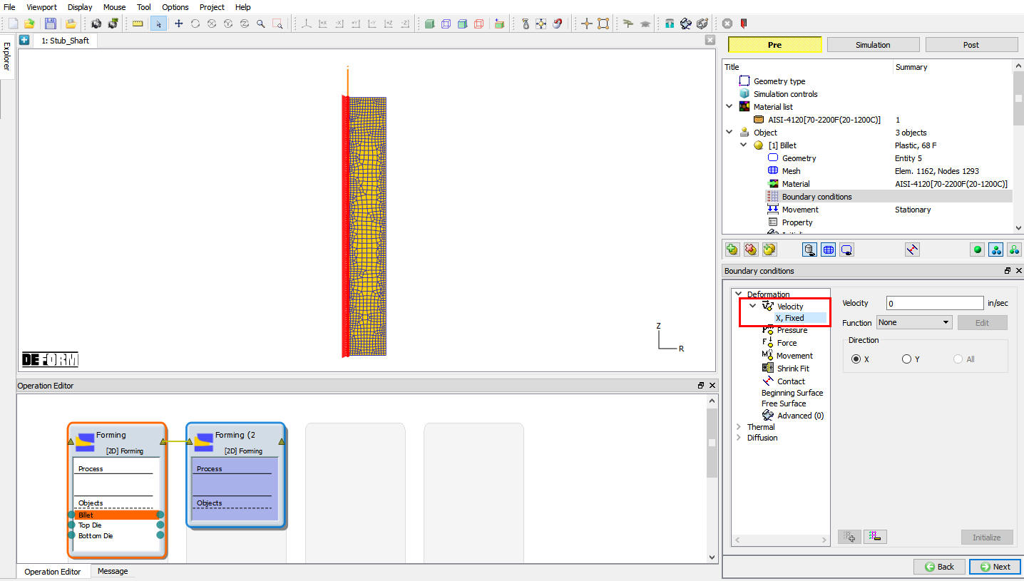
In BCC page, check the default assigned Deformation BCC for Left side of the workpiece in X-Direction as shown in Fig. L25.14., default BCC are assigned automatically due to selection of problem type as axisymmetric. Then click on ![]() up to Top die page.
up to Top die page.
Billet BCC window
Top Die Definition
In Top Die page, change the name of the top die to Punch , Click on ![]() .
.
Import Punch geometry
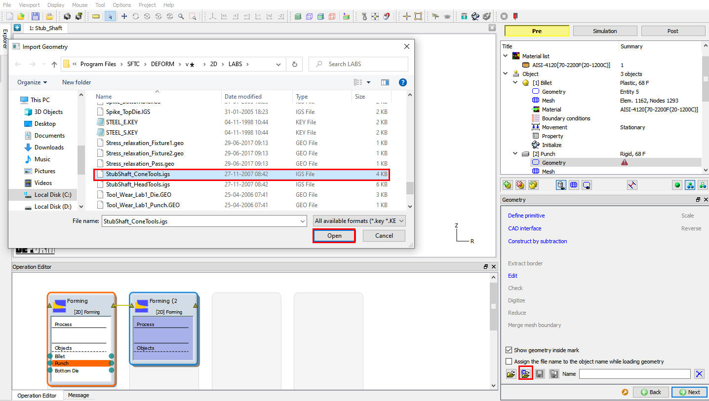
Import StubShaft_ConeTools.igs file using Load Geometry from Library ![]() button as shown in Fig. L25.15. Click
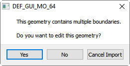
button as shown in Fig. L25.15. Click ![]() for the Multiple boundary popup ( see Fig. L25.16.). When we click ‘Yes’ for the popup edit geometry will open as shown in Fig. L25.17. Deletethe Loop 2 by using
for the Multiple boundary popup ( see Fig. L25.16.). When we click ‘Yes’ for the popup edit geometry will open as shown in Fig. L25.17. Deletethe Loop 2 by using ![]() (see Fig. L25.18.) and click
(see Fig. L25.18.) and click ![]() . Check geometry and click on
. Check geometry and click on ![]() until movement page.
until movement page.
Importing Punch Geometry
Popup to visit edit geometry
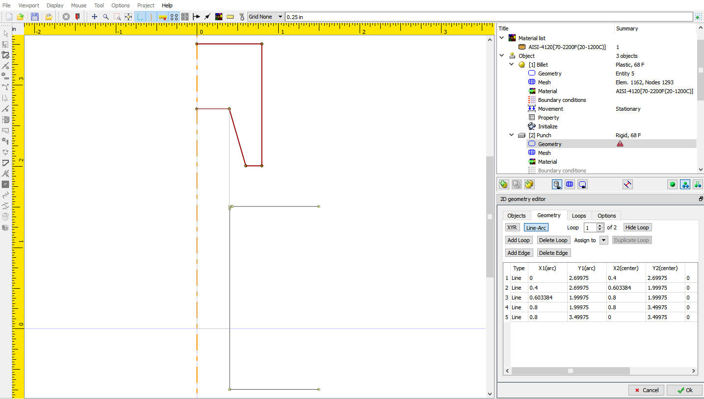
Edit Geometry window
Deleting the Loop 2 from imported geometry
Assign Movement to Top Die
Define a Speed of 10 in/sec in-Y direction for this lab. Then click on ![]() until Bottom Die page.
until Bottom Die page.
Bottom Die Definition
In Bottom die page accept the Object type as Rigid and click on ![]() (see Fig. L25.19.).
(see Fig. L25.19.).
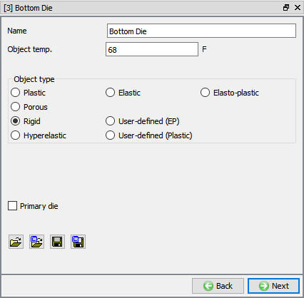
Bottom Die page
Import Bottom Die Geometry
Import StubShaft_ConeTools.igs file using Load Geometry from Library ![]() button. Click
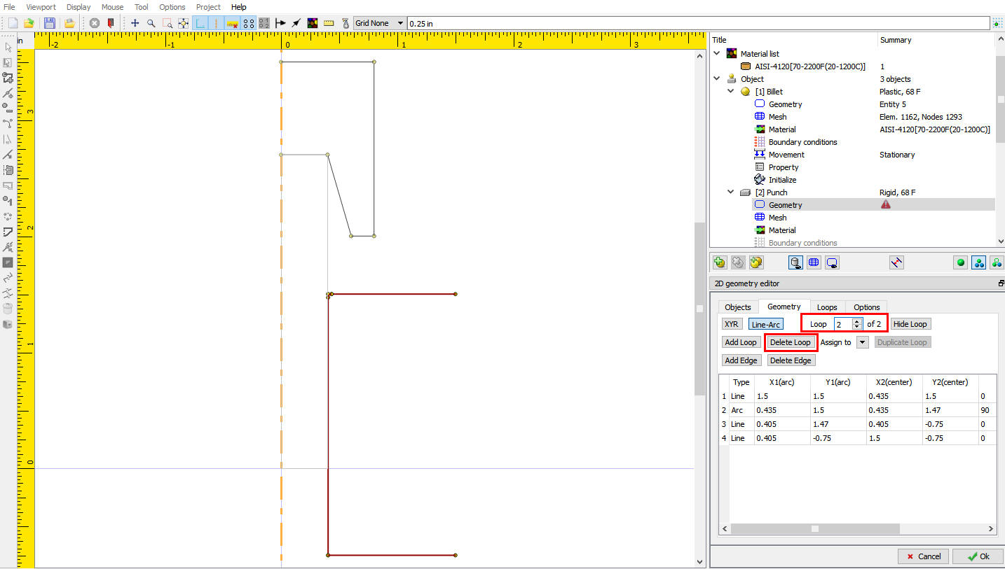
button. Click ![]() for the Multiple boundary popup. When we click ‘Yes’ for the popup edit geometry will open. Deletethe Loop 1 by using
for the Multiple boundary popup. When we click ‘Yes’ for the popup edit geometry will open. Deletethe Loop 1 by using ![]() (see Fig. L25.20.) and click
(see Fig. L25.20.) and click ![]() . Check geometry and click on
. Check geometry and click on ![]() until Object 4 page.
until Object 4 page.
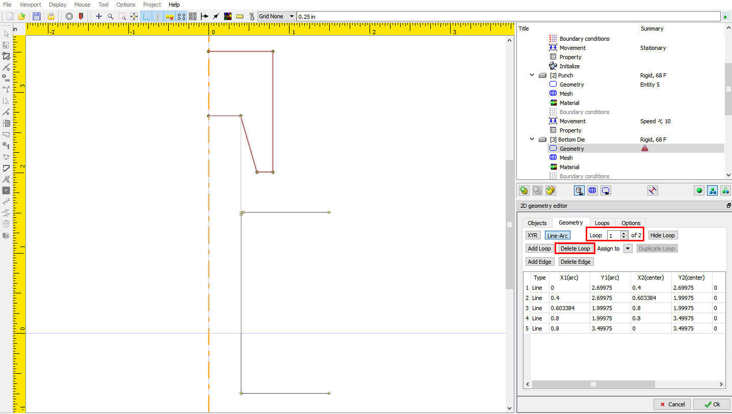
Deleting Loop1 from Imported geometry
Ejector Definition
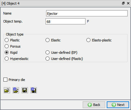
In object 4 window, change the Object 4 Name to Ejector and select Object type as Rigid as shown in Fig. L25.21. Click on ![]() .
.
Ejector object window
Ejector Geometry
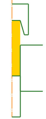
In Ejector geometry window, select the ![]() to visit the edit geometry window and enter the geometry points in the table as shown in Fig. L25.22. and click
to visit the edit geometry window and enter the geometry points in the table as shown in Fig. L25.22. and click ![]() . Check geometry and click on
. Check geometry and click on ![]() until Controls page.
until Controls page.
| X | Y | R |
|---|---|---|
| 0 | -2 | 0 |
| 0.406 | -2 | 0 |
| 0.406 | 0 | 0 |
| 0 | 0 | 0 |
Ejector geometry data

Ejector geometry defining
Controls
Confirm that the workpiece is positioned against the ejector, bottom die is positioned to workpiece and the punch is positioned against the workpiece, see Fig. L25.23. Click on ![]() until Contact page.
until Contact page.
Positioning of the objects
Contact Generation
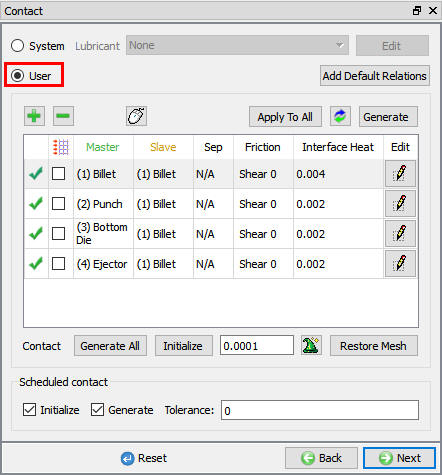
Select user type contact and click on ![]() button. It will add the relationship between the Billet, Punch, Bottom Die and Ejector as shown in Fig. L25.24. As the Dies are Rigid and Billet is plastic, Punch, Bottom Die and Ejector are considered as Master and Billet as Slave. In order to predict the fold during deformation, self contact will be assigned for Billet.
button. It will add the relationship between the Billet, Punch, Bottom Die and Ejector as shown in Fig. L25.24. As the Dies are Rigid and Billet is plastic, Punch, Bottom Die and Ejector are considered as Master and Billet as Slave. In order to predict the fold during deformation, self contact will be assigned for Billet.
Contact Generation page
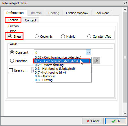
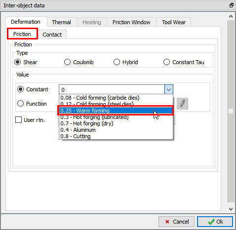
Highlight the Punch – Billet relationship and click the ![]() button to modify the contact conditions. In the friction section of the screen (see Fig. L25.25.), there is a pull-down menu that allows the user to choose the appropriate friction conditions of common forming processes.
button to modify the contact conditions. In the friction section of the screen (see Fig. L25.25.), there is a pull-down menu that allows the user to choose the appropriate friction conditions of common forming processes.
Since this simulation takes place at room temperature and the dies are steel, use the pull down menu and selectCold forming (steel dies) from the list. A friction value of 0.12 will automatically be selected.
Inter-Object data definition window
Click ![]() to go back to contact window, Since the friction conditions are the same for all the object pairs, the
to go back to contact window, Since the friction conditions are the same for all the object pairs, the ![]() button can be used to copy the interface properties from the first relationship to all of the others. After this is done, all relationships will have a friction of 0.12 defined. Use
button can be used to copy the interface properties from the first relationship to all of the others. After this is done, all relationships will have a friction of 0.12 defined. Use ![]() icon to determine a suitable contact tolerance (a value of about 0.00040” will be calculated), then click
icon to determine a suitable contact tolerance (a value of about 0.00040” will be calculated), then click ![]() button to generate contact. Switch to Message tab or Observe status bar to know about the contacts generated. Click on
button to generate contact. Switch to Message tab or Observe status bar to know about the contacts generated. Click on ![]() .
.
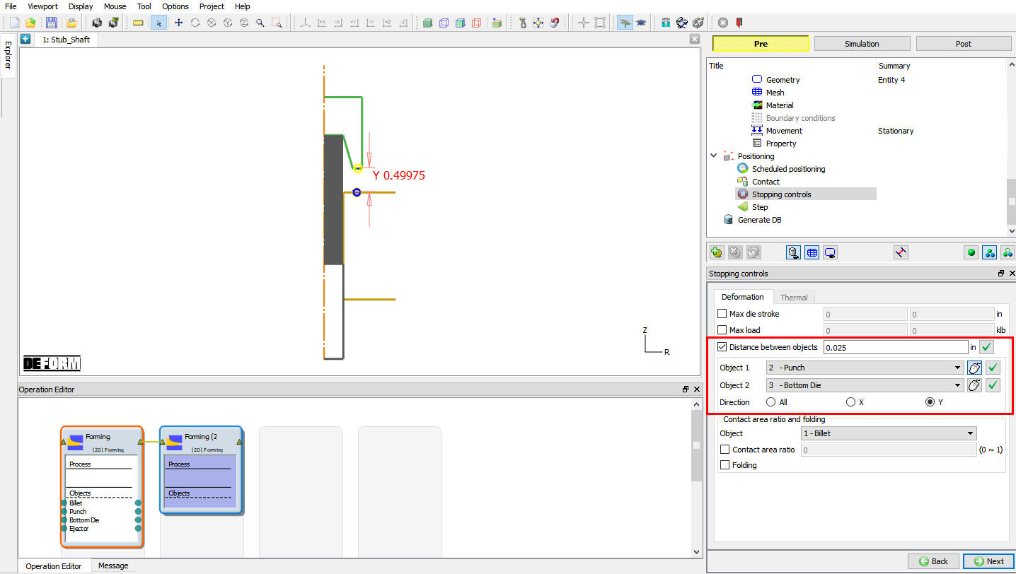
Stopping Controls
We want to stop the simulation when the punch and die are within 0.025” of one another. In the Stopping Controls screen click on ![]() guided mode, check the Distance between objects option. Set the value for this distance to 0.025 ” in the Y direction. Click
guided mode, check the Distance between objects option. Set the value for this distance to 0.025 ” in the Y direction. Click ![]() next to Object 1 and click the bottom of the Punch object in the display. Click
next to Object 1 and click the bottom of the Punch object in the display. Click ![]() next to Object 2 and click the top of the Bottom Die object in the display (see Fig. L25.26.), click on
next to Object 2 and click the top of the Bottom Die object in the display (see Fig. L25.26.), click on ![]() to Step page.
to Step page.
Stopping Controls window
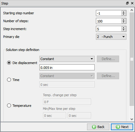
Step Controls
We want the punch to travel 0.5” in 100steps , so each step will be 0.5/100 or 0.005”. In the Step Controls enter the Solution Steps Definition to be With Equal DieDisplacement of 0.005.” set the Number of Simulation Steps to 100 and Step Increment to Save as 5. Set the Punch as Primary Die if not selected automatically (see Fig. L25.27.), click on ![]() .
.
Step Controls window
Generate Database
In Generate DB page. Click the ![]() button to have the program check to see if anything was missed in the problem setup. During the checking process:
button to have the program check to see if anything was missed in the problem setup. During the checking process:
Messages in the red color signify data that needs to be fixed before a simulation can be run (such as when you forget to define any material data).
Click on ![]() button to generate the database. When the program is done writing the database, click on
button to generate the database. When the program is done writing the database, click on ![]() to go to Next operation.
to go to Next operation.
Operation2: Head operation.
Geometry Type
Select 2DAxisymmetricradio button from geometry type page and click on ![]() .
.
Simulation Controls
In Simulation controls uncheck the Heattransfermode check box. Then click on ![]() until Objects page.
until Objects page.
Adding objects
For this operation we required four objects, by default previous operation added four objects are added in object list. if not added objects by default, then add four objects by clicking on ![]() button (see Fig. L25.28.), then click on
button (see Fig. L25.28.), then click on ![]() .
.
Adding Object Window
Workpiece Definition
We will make the Workpiece object as Read Form DB. Select the Read from DB radio button in Workpiece page. Click on ![]() until Top Die page. (See Fig. L25.29.)
until Top Die page. (See Fig. L25.29.)
Workpiece object page
Top Die Definition
In Top Die page, change the object type from Read from DB to Rigid , Click on ![]() .
.
Import Punch geometry:
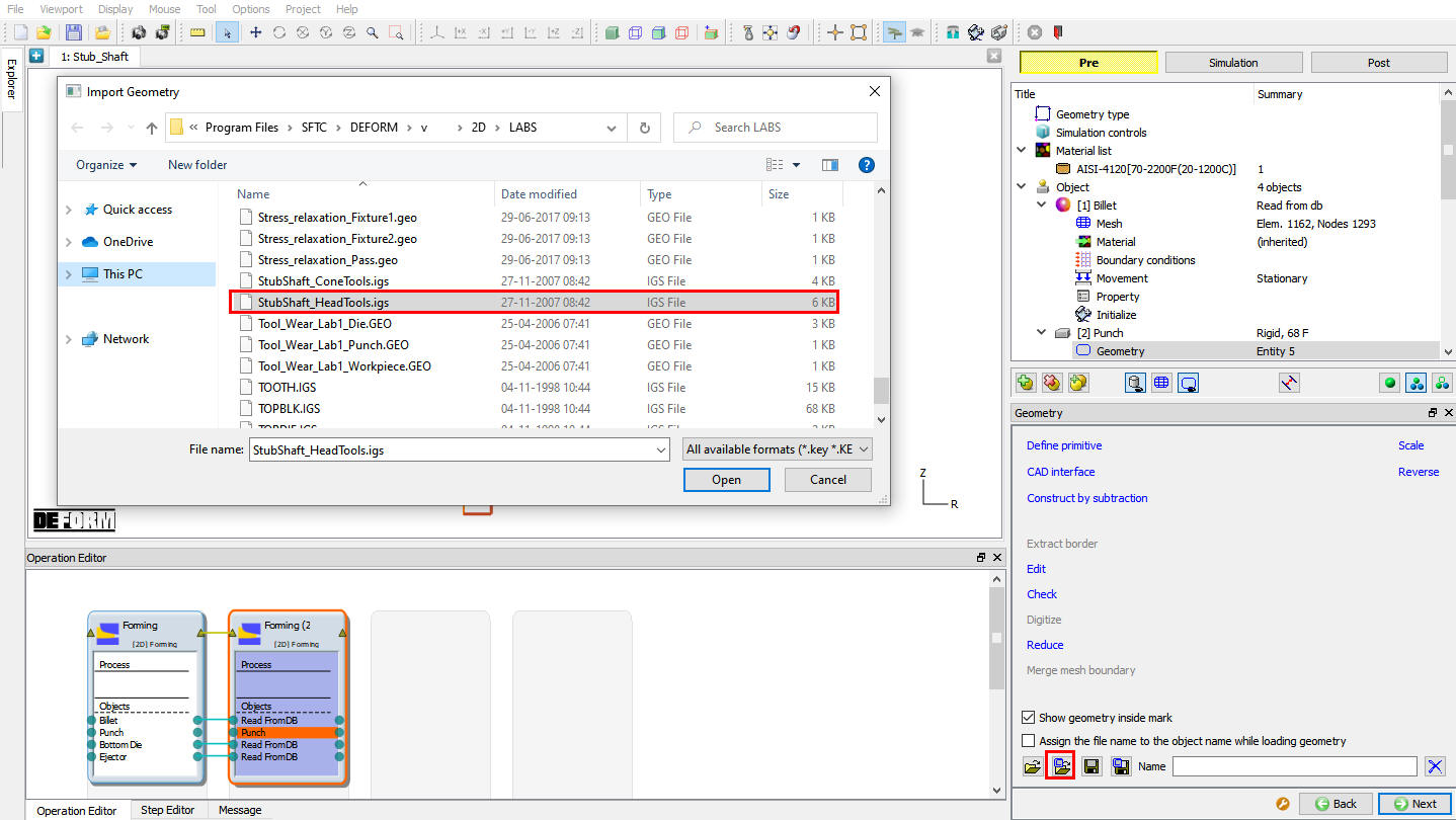
Import StubShaft_HeadTools.igs file using Load Geometry from Library ![]() button as shown in Fig. L25.30. Click
button as shown in Fig. L25.30. Click ![]() for the Multiple boundary popup. When we click ‘yes’ for the popup edit geometry will open. Delete the Loop 1 by using
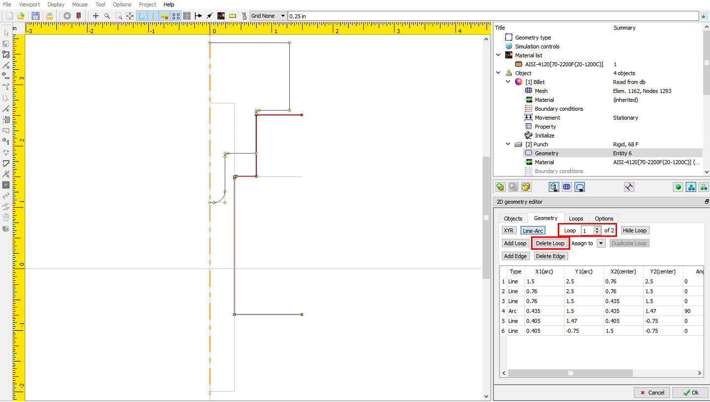
for the Multiple boundary popup. When we click ‘yes’ for the popup edit geometry will open. Delete the Loop 1 by using ![]() (see Fig. L25.31.) and click
(see Fig. L25.31.) and click ![]() . Check geometry and click on
. Check geometry and click on ![]() until movement page.
until movement page.
Load Punch geometry
Edit Geometry window
Assign Movement to Top Die
Define a speed of 10 in/sec in-Y direction for this lab. Then click on ![]() until Bottom Die page.
until Bottom Die page.
Bottom Die Definition
In Bottom die page, change the object type from Read from DB to Rigid** and click on ![]() .
.
Import Bottom Die Geometry
Import StubShaft_HeadTools.igs file using Load Geometry from Library ![]() button. Click
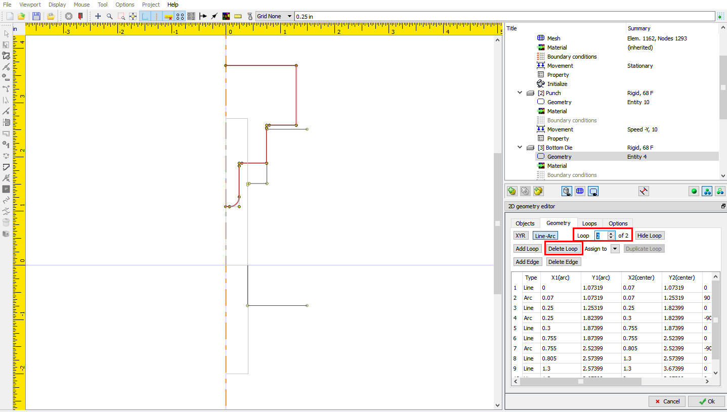
button. Click ![]() for the Multiple boundary popup. When we click ‘yes’ for the popup edit geometry will open. Delete the Loop 2 by using
for the Multiple boundary popup. When we click ‘yes’ for the popup edit geometry will open. Delete the Loop 2 by using ![]() (see Fig. L25.32.) and click
(see Fig. L25.32.) and click ![]() . Check geometry and click on
. Check geometry and click on ![]() until Ejector page.
until Ejector page.
Deleting Loop2 from Imported geometry
Ejector Definition
We will make the Ejector object as Read Form DB. Select the Read from DB radio button in Ejector page. Click on ![]() until Positioning page.
until Positioning page.
Positioning
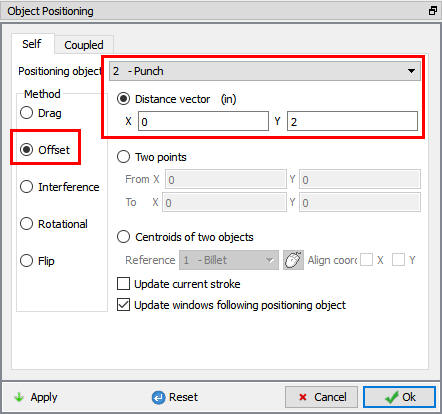
In Object positioning page, position the punch using offsetpositioning(x=0, y=2) towards Y direction (see Fig. L25.33.). Click on ![]() to Scheduled positioning page.
to Scheduled positioning page.
Positioning the Punch
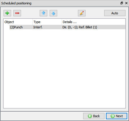
Scheduled Positioning
Using Interference positioning we are positioning the Punch to the Workpiece. In Scheduledpositioning page, Click on ![]() button and select
button and select ![]() radio button. Change the PositioningObject to the Punch and the Reference to the Billet. Change the Approach Direction to -Y and then click
radio button. Change the PositioningObject to the Punch and the Reference to the Billet. Change the Approach Direction to -Y and then click ![]() . (See Fig. L25.34.) Click on
. (See Fig. L25.34.) Click on ![]() .
.
Scheduled Positioning window
Contact Generation
Define the contact relations using the same settings which we defined for the first operation, see 25.1.12.Contact Generation. Click on ![]() .
.
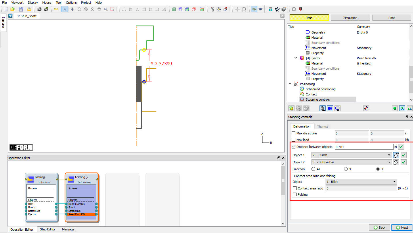
Stopping Controls
We want to stop the simulation when the punch and billet are within 0.401” of one another. In the Stopping Controls screen, check the Distance between objects option. Set the value for this distance to0.401 ” in the Y direction. Click ![]() next to Object 1 and click the Punch object as seen in Fig. L25.35. Click
next to Object 1 and click the Punch object as seen in Fig. L25.35. Click ![]() next to Object 2 and click the Die object as seen in Fig. L25.35.
next to Object 2 and click the Die object as seen in Fig. L25.35.
Distance Between Objects stopping control
We will also specify a maximum load for this part. check the Max load option. Set the Max load to X = 0, Y = 600 as shown in Fig. L25.36. Now if the press load exceeds 600Klb (300Tons), the simulation will stop, even if the distance between tools has not been reached. Click on ![]() .
.

Stop controls page
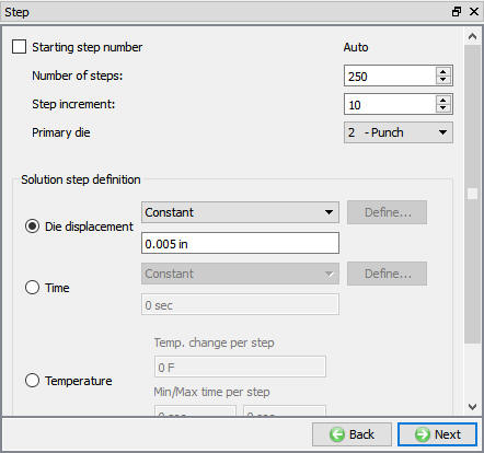
Step Controls
Estimate the total punch travel, which will be roughly 1.25”. We will maintain the stroke per step of 0.005 ”, so the simulation will require about 250 steps (1.25/0.005). Set the Number of Simulation Steps to 250. (See Fig. L25.37.) Click on ![]() .
.
Step Controls window
Generate Database
See the Status in Generate DB page, if we see Input error, check the data missing and complete it, for this lab sequence expect “DB generation is not required for this operation. It will occur at tun time.” message.
Save the project and click on ![]() mode to run the simulation.
mode to run the simulation.
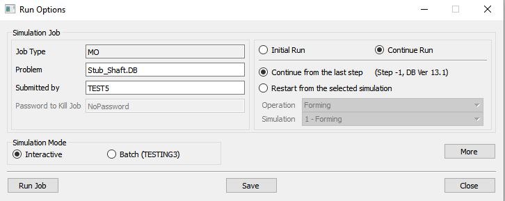
Running simulation
Click on the ![]() action label to open the Run Options dialog as shown in Fig. L25.38. Use the default Continue Run option to select “Continue from the last step ” option and then select the Simulation mode as Interactive and click on
action label to open the Run Options dialog as shown in Fig. L25.38. Use the default Continue Run option to select “Continue from the last step ” option and then select the Simulation mode as Interactive and click on ![]() button to run the simulation.
button to run the simulation.
Run Simulation window
The progress of the simulation can be monitored as it is running by looking at the Simulation Message tab and Simulation Graphics from the Graphics display region in Simulation mode. As long as the ![]() option is checked in Simulation Message tab, which is the default setting, the Message file will refresh automatically.
option is checked in Simulation Message tab, which is the default setting, the Message file will refresh automatically.
The Message file provides information about which simulation step the simulation is currently on and also gives information dealing with how well the simulation is running.
When the simulation is finished without any issues, check the messages in LOG file, when all operation completes we will see messages in LOG file:”MULTIPLE OPERATION COMPLETED”.
Post process the results
After the simulation is completed, Switch to ![]() tab.
tab.
State variables:
From the State variables list, click the Effective strain icon to plot the amount of strain that went into the workpiece. To change the plot settings, you can click on the ![]() Set up icon. In this screen, you can display different kinds of contours (line, shaded or solid) as well as change the variable range that is shown on the contour bar. Using the Settings option, the range of the contour bar can be user-defined. Feel free to experiment with the display of the different state variables and plot options.
Set up icon. In this screen, you can display different kinds of contours (line, shaded or solid) as well as change the variable range that is shown on the contour bar. Using the Settings option, the range of the contour bar can be user-defined. Feel free to experiment with the display of the different state variables and plot options.
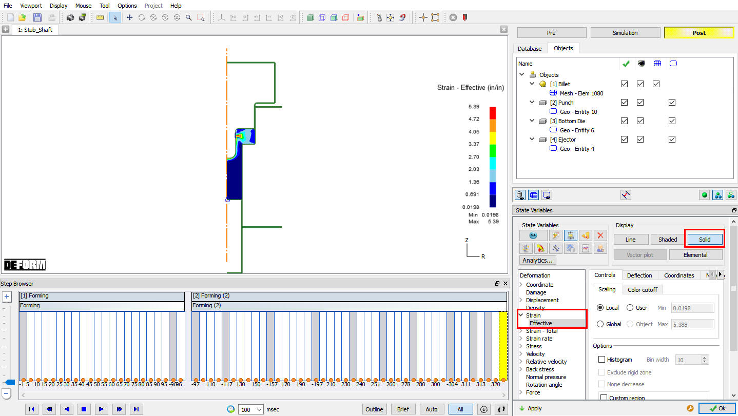
Strain effective plot
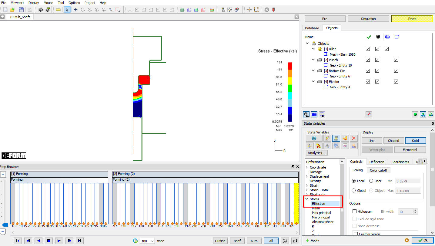
Stress Effective Plot
Flownet
Flownet can be used to create a grid on the starting workpiece shape, the track the distortion of that grid through the simulation.
Click the Flownet ![]() icon to open the Flownet dialog.
icon to open the Flownet dialog.
We will start with a rectangular Flownet. Select “Grid ” and click the ![]() button. Assign a “Spacing ” of 0.1 in the X direction, and 1 in the Y direction. Click
button. Assign a “Spacing ” of 0.1 in the X direction, and 1 in the Y direction. Click ![]() to view the grid. Then click
to view the grid. Then click ![]() . We will not save any data, so click the
. We will not save any data, so click the ![]() button. After the Flownet is calculated, play through the simulation to watch the evolution (see Fig. L25.41.).
button. After the Flownet is calculated, play through the simulation to watch the evolution (see Fig. L25.41.).
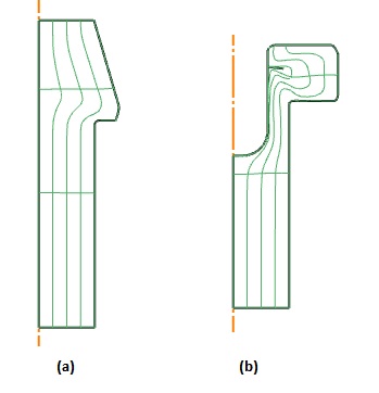
(a) Grid Flownet at second operation first step. (b) Grid Flownet at second operation last step
Tool Stress Analysis
Opening project file
On a Windows machine , go to the ![]() button select DEFORM-v1x.xxx (.xxx indicates version number E.g. v14.0.2) and select DEFORM GUI Main vxx.xx from the menu. The DEFORM GUI Main window will appear.
button select DEFORM-v1x.xxx (.xxx indicates version number E.g. v14.0.2) and select DEFORM GUI Main vxx.xx from the menu. The DEFORM GUI Main window will appear.
Create a new problem either by selecting File![]() New Problem or by clicking the New Problem
New Problem or by clicking the New Problem ![]() icon. The Problem Setup window will appear. Select “ Integrated Manufacturing Process “ radio button and unit system as “English “ using radio button. Define Problem Name as “StubShaft_ToolStress “ and make sure the “Show option dialog ” check box is turned on (if we do not turn on the “Show option dialog” check box, then we will not get the New Project dialog). Then click on
icon. The Problem Setup window will appear. Select “ Integrated Manufacturing Process “ radio button and unit system as “English “ using radio button. Define Problem Name as “StubShaft_ToolStress “ and make sure the “Show option dialog ” check box is turned on (if we do not turn on the “Show option dialog” check box, then we will not get the New Project dialog). Then click on ![]() button to open a new problem using the Deform Integrated Manufacturing Process.
button to open a new problem using the Deform Integrated Manufacturing Process.
Multiple operation wizard will open with the New Project dialog (see Fig. L25.42.), at this point user will be prompted to specify a project name (system will create a separate folder with this project name) and title for this session. In this session we use ‘StubShaft_ToolStress ’ as the project name. Select the copy existing project radio button, select the source location browse button and import the Stub_Shaft.moproj From the previously simulated Stub_shaft Project, turn on the copyDatabase check box, click ![]() for project naming window. Stub_shaft simulation will get imported to ‘StubShaft_ToolStress’ project.
for project naming window. Stub_shaft simulation will get imported to ‘StubShaft_ToolStress’ project.
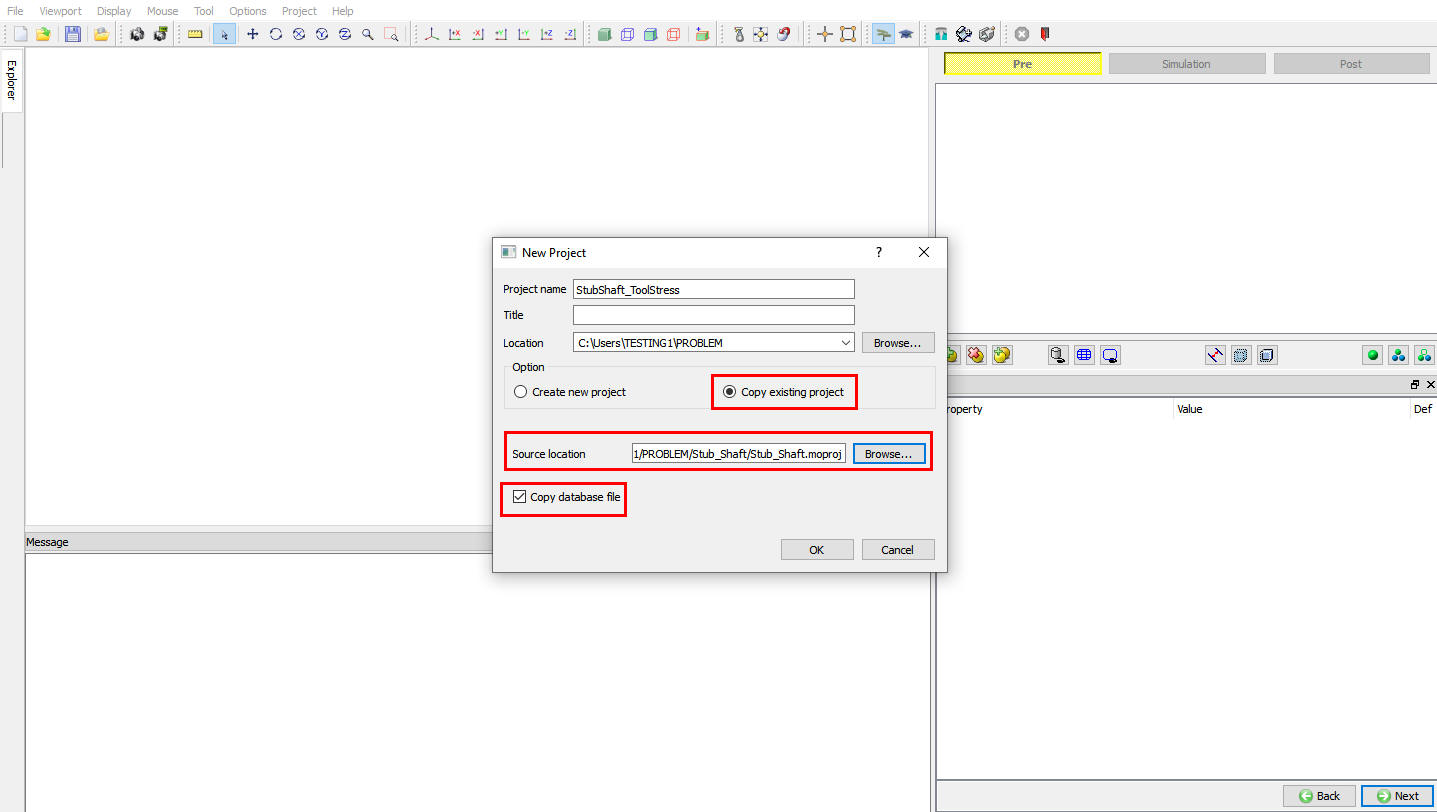
Copying Stub_Shaft project using Copy project option
Add Die stress Operation
Select Die stress 2D operation from the Explorer Operations list and Add the operation by selecting ![]() button or user can also add by drag and drop into the Operation Editor. Now, in Operation Editor,select the Die stress 2D operation.
button or user can also add by drag and drop into the Operation Editor. Now, in Operation Editor,select the Die stress 2D operation.
Add Objects
For this operation we required three objects, hence Keep workpiece, Top Die and Bottom Die objects and delete the Ejector object using ![]() button. Click on
button. Click on ![]() .
.
Object1
By default for object 1, Workpiece (Read object from DB) radio button is selected. Click on ![]() .
.
Top Die
For Top Die, by default for Dies (Elastic) radio button is selected. Click on ![]() until Mesh page.
until Mesh page.
Mesh Generation
Generate the mesh with 2000 elements. Click on ![]() to Material page.
to Material page.
Assign material for Top die
Import a die material AISI-D3 from the material library. ChooseAISI-D3 from the list to assign the material for Top die. Click on ![]() to BCC page.
to BCC page.
Assign Boundary condition for Top die
Next we need to apply boundary conditions to the Top die, so that it does not fly off into space when the forming loads are applied to it. Assign Vy=0 boundary condition on the top edge of the Top die. Click on ![]() to Force interpolation page.
to Force interpolation page.
Force Interpolation
Once the mesh is generated, the forming loads from the workpiece need to be interpolated onto the Top die. Interpolate the force by clicking ![]() option. Click on
option. Click on ![]() until Bottom Die page.
until Bottom Die page.
Bottom Die
For Bottom Die, by default Dies (Elastic) radio button is selected. Click on ![]() until Mesh page.
until Mesh page.
Mesh Generation
Generate the mesh with 2000 elements. Click on ![]() to Material page.
to Material page.
Assign material for Bottom Die
ChooseAISI-D3 from the list to assign the material for Bottom Die. Click on ![]() to BCC page.
to BCC page.
Assign Boundary condition for Bottom Die
Next we need to apply boundary conditions to the Bottom die, so that it does not fly off into space when the forming loads are applied to it.
Assign Vy=0 boundary condition on the bottom Edge of the Bottom Die. Click on ![]() to Force interpolation page.
to Force interpolation page.
Force Interpolation
Once the mesh is generated, the forming loads from the workpiece need to be interpolated onto the Bottom die. Interpolate the force by clicking ![]() option. Click on
option. Click on ![]() until Simulation controls.
until Simulation controls.
Simulation Controls
Define the Numberofstepsas 1 , stepincrementtosave as 1 and timeperstep as 1. Click on ![]() .
.
Generate Database
Click on ![]() action label to check the problem. Generate a database by clicking
action label to check the problem. Generate a database by clicking ![]() action label.
action label.
Running simulation
Once the database has been generated, switch to the Simulation mode by clicking on ![]() button above the operation tree. Click on the
button above the operation tree. Click on the ![]() action label to open the Run Options. Use the default Continue Run option to select “Continue from the last step ” option and then select the Simulation mode as Interactive and click on
action label to open the Run Options. Use the default Continue Run option to select “Continue from the last step ” option and then select the Simulation mode as Interactive and click on ![]() button to run the simulation.
button to run the simulation.
Post Processing
After the simulation is completed, Switch to ![]() tab.
tab.
Using the State Variable option, plot Effective stress and Max Principal stress.
If the effective stress exceeds the yield stress of the material, plastic deformation of the tools will occur.
If the maximum principal stress is large, it may be a site for fatigue failure initiation.
In carbide tools, positive principal stresses, even if they are of relatively small magnitude, may be indicative of fatigue failure initiation.
Note that in this simulation, effective stress is extremely high.
Adding a Shrink ring to the Die
After post processing switch back to the Pre- processor mode by clicking on ![]() tab.
tab.
Add Die stress Operation
Select Die stress 2D operation from the Explorer Operations list and Add the operation by selecting ![]() button or user can also add by drag and drop into the Operation Editor.
button or user can also add by drag and drop into the Operation Editor.
Now, in Operation Editor select the added Die stress 2D operation.
Add Objects
For this operation we required four objects, hence in Object window add another one object by clicking ![]() button. Click on
button. Click on ![]() until Object 4 page.
until Object 4 page.
Defining Ring
In Object4 page, change the object name to Ring and accept theDies (Elastic) object type. Click on ![]() .
.
Case Geometry definition
Select the ![]() and define a hollowcylinder with Innerradius as 1.5 “, Outerradius as 3.5 “ and height will be 3.25 ”, click
and define a hollowcylinder with Innerradius as 1.5 “, Outerradius as 3.5 “ and height will be 3.25 ”, click ![]() . Click on
. Click on ![]() to Mesh page.
to Mesh page.
Mesh generation
Generate the mesh with 2000 elements. Click on ![]() .
.
Assign material for Case
Choose AISI-D3 from the list to assign the material for Ring. Click on ![]()
Boundary conditions
Assign Velocity Vy=0 along the bottom edge of the Ring.
Assign a shrink fit of 0.007” along the ID of the Ring. Click on ![]() until Positioning page.
until Positioning page.
Positioning objects
Using offset with Two points , make the Ring as the positioning object. Click on the bottom inside corner of the ring , then thebottom outside corner of the Bottom die. DEFORM should pick the points From (1.5, 0) To (1.5, -0.75). If these are not the exact values in the object positioning window, edit the values to make them exact. Click the ![]() button to move the Ring. Then click
button to move the Ring. Then click ![]() to exit object positioning. Click on
to exit object positioning. Click on ![]() until Contact page.
until Contact page.
Contact generation
We will make the Bottom Die as Slave, and the Ring as Master. click on ![]() button to add Ring - Bottom Die relation, select Master object as Ring and Slave object as Bottom Die, define Friction value as 0.12 and generate contact by click
button to add Ring - Bottom Die relation, select Master object as Ring and Slave object as Bottom Die, define Friction value as 0.12 and generate contact by click ![]() button. User should see a line of dots along the boundary. Click on
button. User should see a line of dots along the boundary. Click on ![]() .
.
Simulation Controls
Define the Number of steps as 1, step increment to save as 1 and time per step as 1. Click on ![]() to generate Database page.
to generate Database page.
Generate Database
Click on ![]() action label to check the problem. Generate a database by clicking
action label to check the problem. Generate a database by clicking ![]() action label.
action label.
Running simulation
Once the database has been generated, switch to the Simulation mode by clicking on ![]() button above the operation tree. Click on the
button above the operation tree. Click on the ![]() action label to open the Run Options. Use the default Continue Run option to select “Continue from the last step ” option and then select the Simulation mode as Interactive and click on
action label to open the Run Options. Use the default Continue Run option to select “Continue from the last step ” option and then select the Simulation mode as Interactive and click on ![]() button to run the simulation.
button to run the simulation.
Post Processing
Compare the stresses in first die stress operation (no shrink ring) with second die stress operation (with shrink ring). Stresses in second die stress operation should be lower, but still quite high. Use the state variable properties and use global rather than local scaling.
Note the stresses in the case are in the order of 1000KSI or higher. Adding a heavier interference fit will likely cause the ring to yield.
Simulating Thermal Effects
In the next simulation, we will repeat the process as a warm forging. We will simulate transfer from the heat transfer, resting on the die, and the cone-forging blow.
Transfer in Air
Opening project file
On a Windows machine , go to the ![]() button select DEFORM-v1x.xxx (.xxx indicates version number E.g. v14.0.2) and select DEFORM GUI Main vxx.xx from the menu. The DEFORM GUI Main window will appear.
button select DEFORM-v1x.xxx (.xxx indicates version number E.g. v14.0.2) and select DEFORM GUI Main vxx.xx from the menu. The DEFORM GUI Main window will appear.
Create a new problem either by selecting File![]() New Problem or by clicking the New Problem
New Problem or by clicking the New Problem ![]() icon. The Problem Setup window will appear. Select “ Integrated Manufacturing Process “ radio button and unit system as “English “ using radio button. Define Problem Name as “Stub_shaft_Warm “ and make sure the “Show option dialog ” check box is turned on (if we do not turn on the “Show option dialog” check box, then we will not get the New Project dialog). Then click on
icon. The Problem Setup window will appear. Select “ Integrated Manufacturing Process “ radio button and unit system as “English “ using radio button. Define Problem Name as “Stub_shaft_Warm “ and make sure the “Show option dialog ” check box is turned on (if we do not turn on the “Show option dialog” check box, then we will not get the New Project dialog). Then click on ![]() button to open a new problem using the Deform Integrated Manufacturing Process.
button to open a new problem using the Deform Integrated Manufacturing Process.
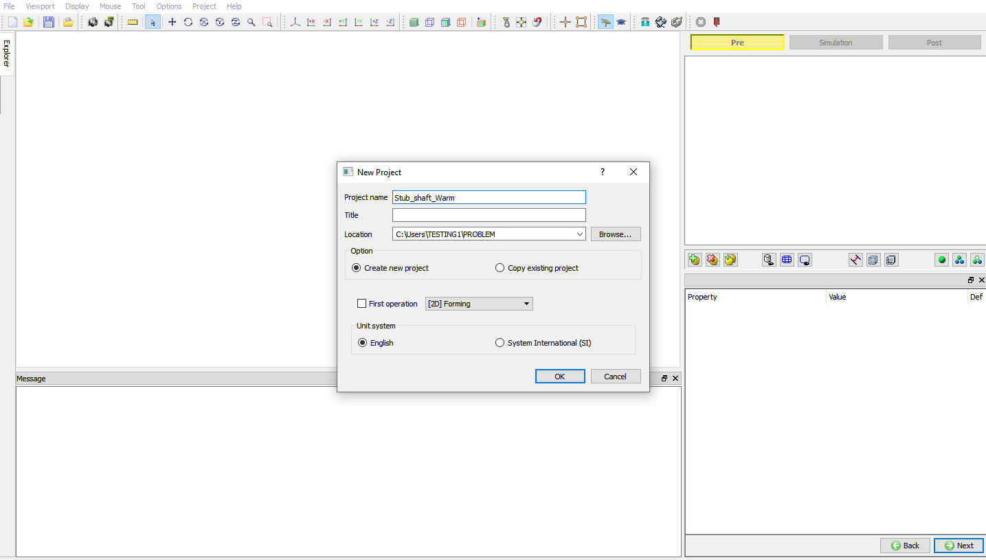
MO wizard will open along with project naming window (see Fig. L25.43.). In the field of project name, in this session we use ‘**Stub_shaft_Warm** ’ as the project name. Click on ![]() to continue to open the operation.
to continue to open the operation.
Problem defining window
Add operations
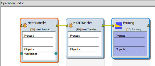
Add two 2D Heat Transfer operations and one2D Forming operation from Operation list in Explorer as shown in Fig. L25.44. Operation can be added by clicking on ![]() button next to respective operation or user can also add the operation by dragging and dropping the operation into Operation Editor region.
button next to respective operation or user can also add the operation by dragging and dropping the operation into Operation Editor region.
Adding operations
Importing the DB
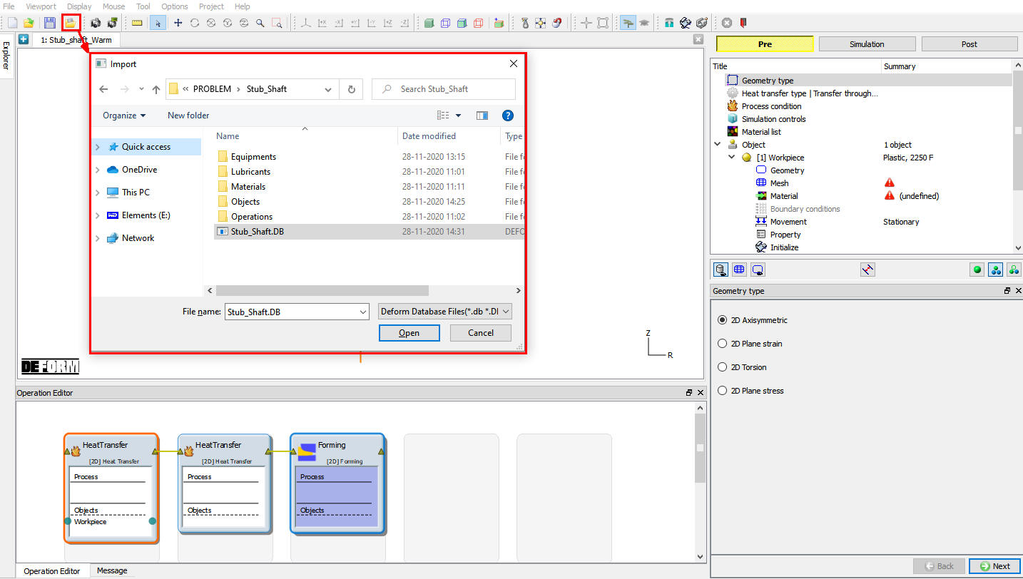
After adding all Three operations, import previously simulated Stub_Shaft.DB , select the first step and click ![]() as shown in Fig. L25.46.
as shown in Fig. L25.46.
Importing DB

Step selection window
Geometry Type
In this lab we will be using Axisymmetric geometries, So select 2DAxisymmetric radio button from geometry type page and click on ![]() . (See Fig. L25.47.)
. (See Fig. L25.47.)
Axisymmetric Geometry type selection
Selecting Heat Transfer Type
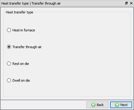
Select Heat Transfer Type as “Transfer through air “ for first operation as shown in Fig. L25.48. This will set the default heat transfer settings for heating operation. Click on ![]() .
.
Heat transfer type selection for Furnace Heating operation
Set Process Conditions
Define Heatingtime as 5 sec at 68F furnace temperature or environment temperature as shown in Fig. L25.49 and click on ![]() .
.

Process condition window
Select Simulation Controls
Keep only Heat Transfer mode checked as only heat transfer is modelling as shown in Fig. L25.50. and click on ![]() until Billet page.
until Billet page.
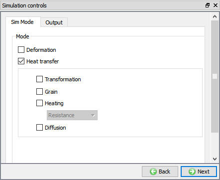
Simulation Controls settings for Furnace Heating
Defining Billet
In Billet object window accept the object type as ‘Plastic ’ and change the object temperature to 1750°F as shown in** Fig. L25.51. We will use the same geometry and mesh from the cold forming simulation. Click on ![]() until Punch page.
until Punch page.
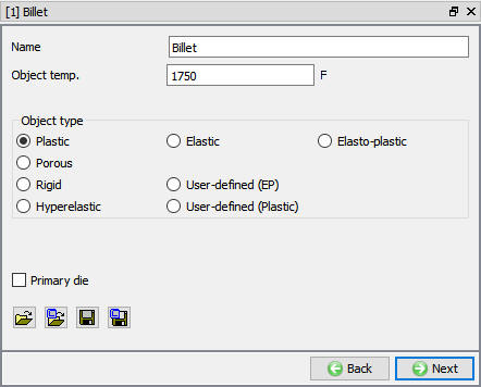
Billet Definition Page
Punch Definition
In Punch page define the object temp to 300F and click on ![]() until Mesh page.
until Mesh page.
Mesh Generation
Generate the mesh for the existing geometry. Generate a mesh with the default number of elements (see Fig. L25.52.). Click on ![]() to Material page.
to Material page.
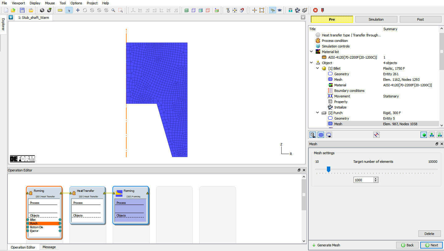
Punch Mesh generation
Assigning Material for the Punch
Import a die material AISI-H-13 from the material library. Choose AISI-H-13 from the list to assign the material for Punch. Click on ![]() until Movement page.
until Movement page.
Deleting Movement definition
Delete the Punch existing movement by using ![]() button in the top die movement page. Click on
button in the top die movement page. Click on ![]() until Bottom Die page.
until Bottom Die page.
Bottom die Definition
In Bottom die page define the object temp to 300F and click on ![]() until Mesh page.
until Mesh page.
Mesh Generation
Generate the mesh for the existing geometry. Generate a mesh with the default number of elements. Click on ![]() to Material page.
to Material page.
Assigning Material for the Bottom die
Choose AISI-H-13 from the list to assign the material for Bottom die. Click on ![]() until Ejector page.
until Ejector page.
Ejector Definition
In Ejector page define the object temp to 300F and click on ![]() until Mesh page.
until Mesh page.
Mesh Generation
Generate the mesh for the existing geometry. Generate a mesh with the default number of elements. Click on ![]() to Material page.
to Material page.
Assigning Material for the Ejector
Choose AISI-H-13 from the list to assign the material for Ejector. Click on ![]() until Positioning page.
until Positioning page.
Positioning
Click on ![]() button. Use
button. Use ![]() to move the Punch3 inches in the “Y” direction. Also move the workpiece 2 inches in the “Y” direction. Click on to
to move the Punch3 inches in the “Y” direction. Also move the workpiece 2 inches in the “Y” direction. Click on to ![]() exit the positioning menu. Click on
exit the positioning menu. Click on ![]() until Step controls window.
until Step controls window.
Step control
Set the number of simulation steps as 50 at 0.1sec each and saving every 5 steps (See Fig. L25.53.). Advanced Simulation controls settings are available in expert mode (![]() ). Click on
). Click on ![]() to proceed to the database generation stage.
to proceed to the database generation stage.
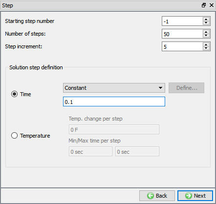
Step controls settings
Generate Database
In Generate DB page. Click the ![]() button to have the program check to see if anything was missed in the problem setup. During the checking process:
button to have the program check to see if anything was missed in the problem setup. During the checking process:
Messages in the red color signify data that needs to be fixed before a simulation can be run (such as when you forget to define any material data).
Click on ![]() button to generate the database. When the program is done writing the database, click on
button to generate the database. When the program is done writing the database, click on ![]() to go to Next operation.
to go to Next operation.
Rest on die
Selecting Heat Transfer Type
Select Rest on die transfer type for second operation. This will set the default heat transfer settings for heating operation. Click on ![]() to continue.
to continue.
Set Process Conditions
Define Resting time as 1 second with an environment temperature of 68° F as shown in Fig. L25.54. and click on ![]() to continue.
to continue.
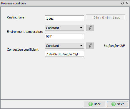
Process condition window
Select Simulation Controls
Keep only Heat Transfer mode checked as only heat transfer is modelling and click on ![]() .
.
Defining Objects
By default all the objects will be in Read from DB, accept the default object types and click on ![]() until scheduled positioning page.
until scheduled positioning page.
Scheduled positioning
click on ![]() (Add) button and use
(Add) button and use ![]() Positioning option to position the Billet against the Ejector in “ -Y” direction. Click on
Positioning option to position the Billet against the Ejector in “ -Y” direction. Click on ![]() .
.
Contact Generation
Select user type contact and click on ![]() (Add relationship) button twice and select Bottomdie as Master and Billet as Slave for first relation and for second relation select Ejector as Master and Billet as Slave as shown in Fig. L25.55.
(Add relationship) button twice and select Bottomdie as Master and Billet as Slave for first relation and for second relation select Ejector as Master and Billet as Slave as shown in Fig. L25.55.
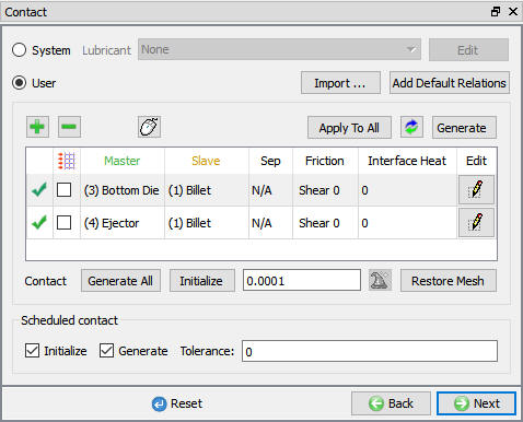
Inter-object relationship between workpiece and bottom die
Click on Bottom die- Billet![]() (Edit) relationship button and select the pull down option “Free Resting “ in the thermal section to define the inter-object heat transfer coefficient as shown in Fig. L25.56. Click
(Edit) relationship button and select the pull down option “Free Resting “ in the thermal section to define the inter-object heat transfer coefficient as shown in Fig. L25.56. Click ![]() to close the Editing window. Then click on
to close the Editing window. Then click on ![]() button to copy the interface properties from the first relationship to the other relationships. It will generate the inter-object contact at the beginning of the resting operation while simulating. Click on
button to copy the interface properties from the first relationship to the other relationships. It will generate the inter-object contact at the beginning of the resting operation while simulating. Click on ![]() until step controls window.
until step controls window.
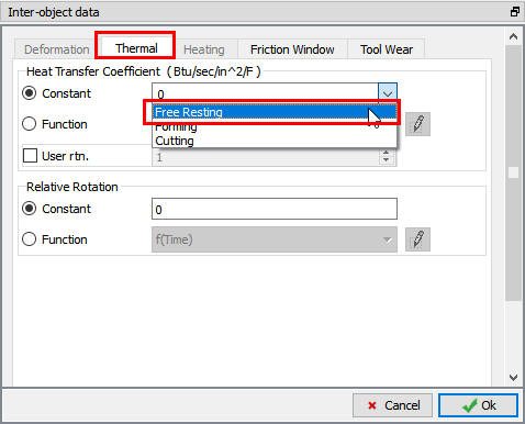
Inter-object Heat transfer coefficient selection for resting
Step control
Set the number of simulation steps as 50 at 0.1 sec each and saving every 5 steps. Advanced Simulation controls settings are available in expert mode (![]() ). Click on
). Click on ![]() to proceed to the database generation stage.
to proceed to the database generation stage.
Generate Database
See the Status in Generate DB page. If we see Input error, check the data missing and complete it. For this lab sequence we expect to see “DB generation is not required for this operation. It will occur at run time.” message. click on ![]() to go to Next operation.
to go to Next operation.
Form cone Operation
For the forming operation turnon the Deformation check box along with Heat transfer in Simulation controls page. Click on ![]() .
.
Defining the objects
In the Objects page, by default all four objects are added in list. If not, add four objects by using ![]() button and make all four objects as Read from DB objects by visiting every object page. (See Fig. L25.57.)
button and make all four objects as Read from DB objects by visiting every object page. (See Fig. L25.57.)
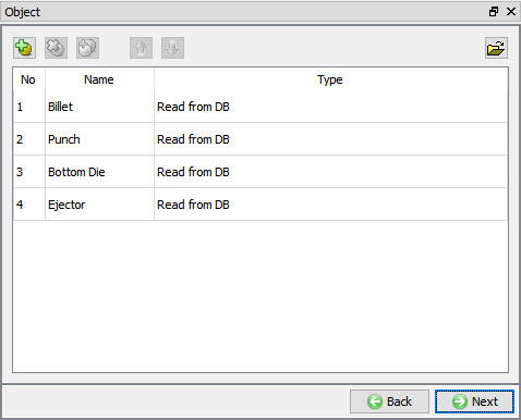
Objects page
Punch Definition
Defining the Punch movement
Define a speed of 10 in/sec in -Y direction for the Punch object. Then click on ![]() until Scheduled positioning page.
until Scheduled positioning page.
Scheduled Positioning
In scheduled Positioning page, click on ![]() (Add) button and select the ‘Positioningobject ’ as Punch , method as ‘Interference ’ with respect to ‘Billet ’ in the -Y direction. Click on
(Add) button and select the ‘Positioningobject ’ as Punch , method as ‘Interference ’ with respect to ‘Billet ’ in the -Y direction. Click on ![]() to continue.
to continue.
Contact Generation
Select user type contact and click on ![]() button. It will add the relationship between the Billet, Punch, Bottom Die and Ejector. As the Dies are Rigid and Billet is plastic, Top and Bottom Dies are considered as Master and Billet as Slave.
button. It will add the relationship between the Billet, Punch, Bottom Die and Ejector. As the Dies are Rigid and Billet is plastic, Top and Bottom Dies are considered as Master and Billet as Slave.
Highlight the Punch – Billet relationship and click the ![]() button to modify the contact conditions. In the friction section of the screen (see Fig. L25.58.), there is a pull-down menu that allows the user to choose the appropriate friction conditions of common forming processes.
button to modify the contact conditions. In the friction section of the screen (see Fig. L25.58.), there is a pull-down menu that allows the user to choose the appropriate friction conditions of common forming processes.
Since this is hot forming simulation and the dies are steel, use the pull down menu and select Warm forming from the list. A friction value of 0.25 will automatically be selected. Switch to Thermaltab and select forming and select the pull down option “Forming “ to define the inter-object heat transfer coefficient.
Inter-object friction coefficient definition window
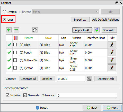
Click ![]() to go back to Inter-Object window, since the friction conditions are the same for all the object pairs, the
to go back to Inter-Object window, since the friction conditions are the same for all the object pairs, the ![]() button can be used to copy the interface properties from the first relationship to all of the others. After this is done, all relationships will have a friction of 0.25 and Interface heat transfer as 0.004 as shown in Fig. L25.59. Since the contact will initialize and generate while generating database. Click on
button can be used to copy the interface properties from the first relationship to all of the others. After this is done, all relationships will have a friction of 0.25 and Interface heat transfer as 0.004 as shown in Fig. L25.59. Since the contact will initialize and generate while generating database. Click on ![]() to continue.
to continue.
Inter-Object relationship definition for forming operation
Stopping Controls
Set the stopping controls as explained in the section Stopping controls 25.1.13.
Step Controls
Set the step controls as explained in the section Step controls 25.1.14.
Generate Database
See the Status in Generate DB page. If we see Input error, check the data missing and complete it. For this lab sequence we expect to see “DB generation is not required for this operation. It will occur at run time.” message.
Running simulation
Switch to the Simulation mode by clicking on ![]() button above the operation tree. Click on the
button above the operation tree. Click on the ![]() action label to open the Run Options. Use the default Continue Run option to select “Continue from the last step ” option and then select the Simulation mode as Interactive and click on
action label to open the Run Options. Use the default Continue Run option to select “Continue from the last step ” option and then select the Simulation mode as Interactive and click on ![]() button to run the simulation.
button to run the simulation.
Post process the results
After the simulation is completed, Switch to ![]() tab.
tab.
check the load in the post-processor.
How does the load compare to the cold forming case?
Point track temperature at several points in the head of the part. What happens to the temperature as the part is formed?
Warm Stub shaft with Mechanical press movement
Opening project file
On a Windows machine , go to the ![]() button select DEFORM-v1x.xxx (.xxx indicates version number E.g. v14.0.2) and select DEFORM GUI Main vxx.xx from the menu. The DEFORM GUI Main window will appear.
button select DEFORM-v1x.xxx (.xxx indicates version number E.g. v14.0.2) and select DEFORM GUI Main vxx.xx from the menu. The DEFORM GUI Main window will appear.
Create a new problem either by selecting File![]() New Problem or by clicking the New Problem
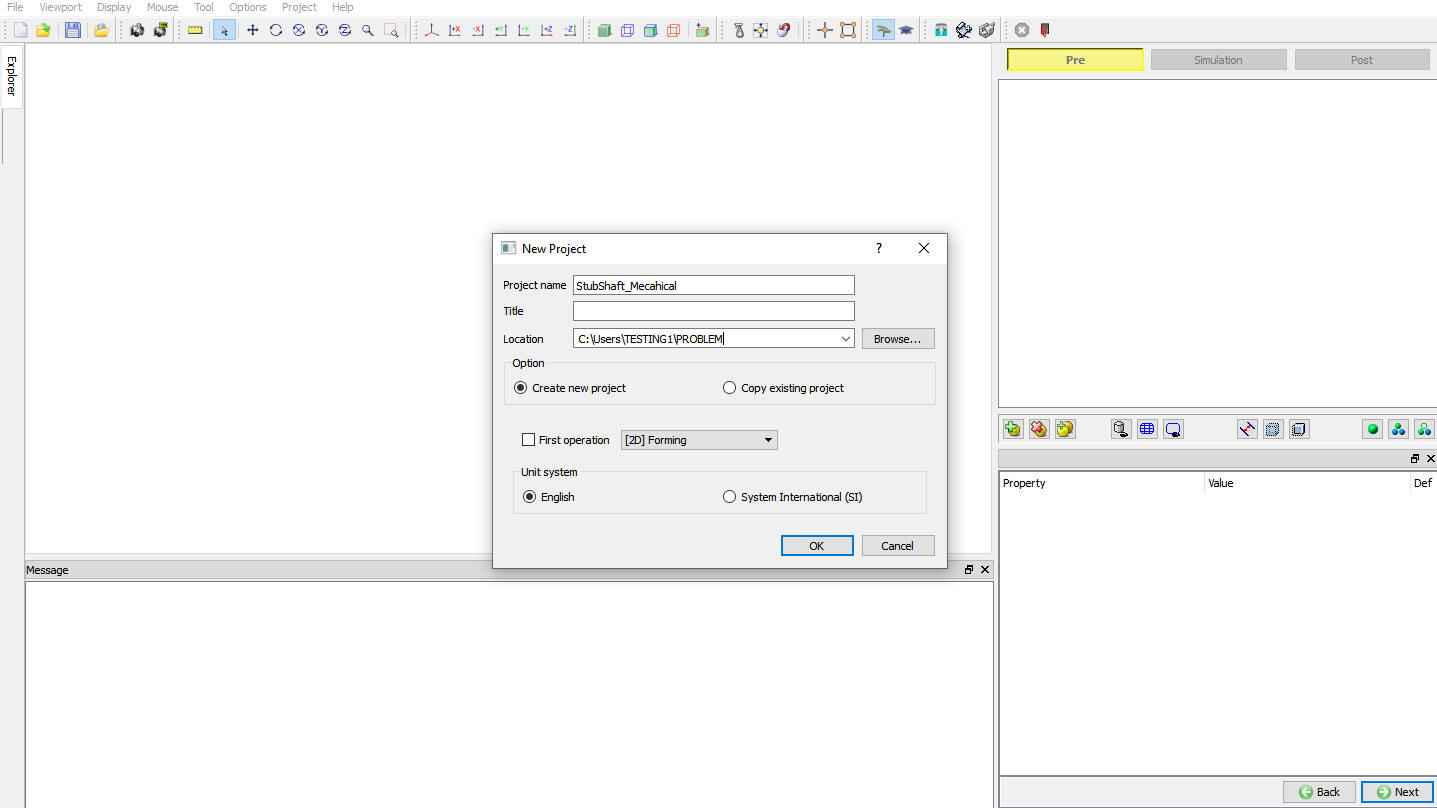
New Problem or by clicking the New Problem ![]() icon. The Problem Setup window will appear. Select “ Integrated Manufacturing Process “ radio button and unit system as “English “ using radio button. Define Problem Name as “StubShaft_Mecahical “ and make sure the “Show option dialog ” check box is turned on (if we do not turn on the “Show option dialog” check box, then we will not get the New Project dialog). Then click on
icon. The Problem Setup window will appear. Select “ Integrated Manufacturing Process “ radio button and unit system as “English “ using radio button. Define Problem Name as “StubShaft_Mecahical “ and make sure the “Show option dialog ” check box is turned on (if we do not turn on the “Show option dialog” check box, then we will not get the New Project dialog). Then click on ![]() button to open a new problem using the Deform Integrated Manufacturing Process.
button to open a new problem using the Deform Integrated Manufacturing Process.
MO wizard will open along with project naming window (see Fig. L25.60.). In the field of project name, in this session we use ‘**StubShaft_Mecahical** ’ as the project name. Click on ![]() to continue to open the operation.
to continue to open the operation.
Problem defining window
Add Forming Operation
Add 2D Forming operation from the Explorer Operations list. Add the operation by clicking on ![]() button or user can also add by drag and drop into the Operation Editor.
button or user can also add by drag and drop into the Operation Editor.
Importing the DB
After adding 2D Forming operation, import previously simulated Stub_shaft_Warm.DB , select the first step of the third operation and click ![]() . Click on
. Click on ![]() until Punch Movement page.
until Punch Movement page.
Punch Definition
Punch Movement Definition
Select the movement type as Mechanical press. The total stroke is the movement of the ram from top dead center to bottom dead center (or back to front, for a horizontal press).
We will specify atotal stroke of 10 ”.
The forging stroke is the distance the punch travels from the time it contacts the workpiece until it reaches bottom dead center. For this simulation, theforging stroke will be 0.5 ”.
The number of Cycles/second is the speed of the flywheel. On a header, or a press without a clutch, it will equal the Cycles/second of the press. On a press with a clutch, it will be Flywheel RPM / 60 rev/sec or cycles/sec.
We will specify 1.1 Cycles / sec.
We will keep rest of the settings as imported. click on ![]() until DB Generation page.
until DB Generation page.
Generate DB
Check the data and generate the DB. After generating DB switch to ![]() mode to run the simulation.
mode to run the simulation.
Running simulation
Click on the ![]() action label to open the Run Options. Use the default Continue Run option to select “Continue from the last step ” option and then select the Simulation mode as Interactive and click on
action label to open the Run Options. Use the default Continue Run option to select “Continue from the last step ” option and then select the Simulation mode as Interactive and click on ![]() button to run the simulation.
button to run the simulation.
After simulation complete, switch to ![]() tab.
tab.
Post processor
In Step Browser click on ![]() button to view all steps. Play through the steps to see the deformation.
button to view all steps. Play through the steps to see the deformation.
Go to the load-stroke ![]() plot and plot the punch velocity vs time. Plot the load vs. time.
plot and plot the punch velocity vs time. Plot the load vs. time.
User can compare the maximum load using the press model to the maximum load using the constant speed approximation.
Warm Stub shaft with Hydraulic press movement
Opening project file
On a Windows machine , go to the ![]() button select DEFORM-v1x.xxx (.xxx indicates version number E.g. v14.0.2) and select DEFORM GUI Main vxx.xx from the menu. The DEFORM GUI Main window will appear.
button select DEFORM-v1x.xxx (.xxx indicates version number E.g. v14.0.2) and select DEFORM GUI Main vxx.xx from the menu. The DEFORM GUI Main window will appear.
Create a new problem either by selecting File![]() New Problem or by clicking the New Problem
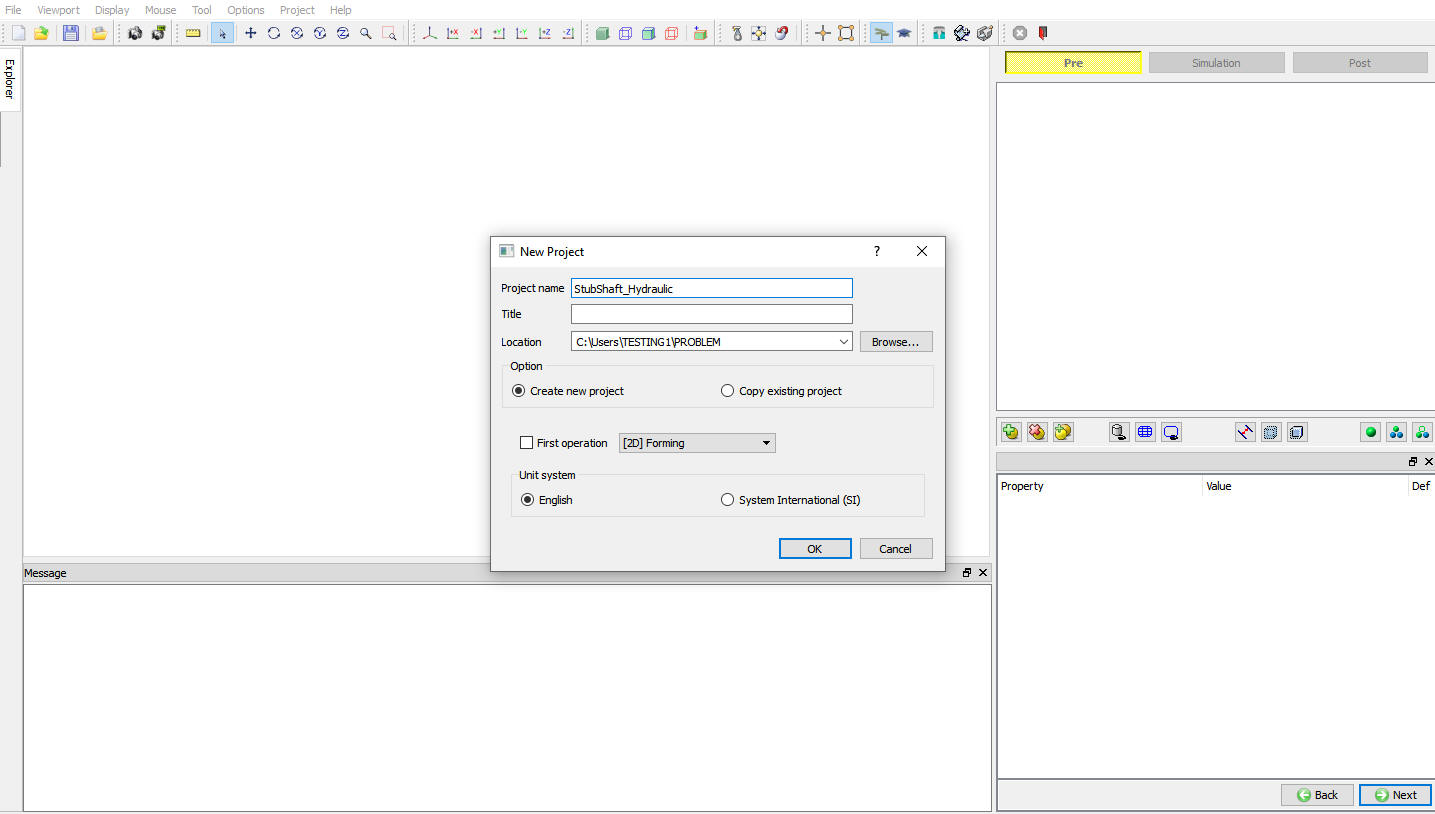
New Problem or by clicking the New Problem ![]() icon. The Problem Setup window will appear. Select “ Integrated Manufacturing Process “ radio button and unit system as “English “ using radio button. Define Problem Name as “StubShaft_Hydraulic “ and make sure the “Show option dialog ” check box is turned on (if we do not turn on the “Show option dialog” check box, then we will not get the New Project dialog). Then click on
icon. The Problem Setup window will appear. Select “ Integrated Manufacturing Process “ radio button and unit system as “English “ using radio button. Define Problem Name as “StubShaft_Hydraulic “ and make sure the “Show option dialog ” check box is turned on (if we do not turn on the “Show option dialog” check box, then we will not get the New Project dialog). Then click on ![]() button to open a new problem using the Deform Integrated Manufacturing Process.
button to open a new problem using the Deform Integrated Manufacturing Process.
MO wizard will open along with project naming window (see Fig. L25.61.). In the field of project name, in this session we use ‘**StubShaft_Hydraulic** ’ as the project name. Click on ![]() to continue to open the operation.
to continue to open the operation.
Problem defining window
Add Forming Operation
Add 2D Forming operation from the Explorer Operations list. Add the operation by clicking on ![]() button or user can also add by drag and drop into the Operation Editor.
button or user can also add by drag and drop into the Operation Editor.
Importing the DB
After adding 2D Forming operation, import previously simulated Stub_shaft_Warm.DB , select the first step of the third operation and click ![]() . Click on
. Click on ![]() until Punch Movement page.
until Punch Movement page.
Punch Movement Definition
Select the movement type as Hydraulic press. For this simulation, check the Power limit box, click the ![]() button, and define the following values.
button, and define the following values.
| Force | Speed |
|---|---|
| 0 | 1.5 |
| 20 | 1.3 |
| 25 | 1.1 |
| 30 | 0.7 |
| 35 | 0.25 |
| 38 | 0 |
This means that the max speed of the press – unloaded – is 1.5 in/sec.
The max load of the press is 38 Klb at final step (stall speed.)
At 25 Klb, the press can maintain 1.1 in/sec.
Note that these load values are constructed to illustrate press behavior in this tutorial. The loads are quite small.
Defineconstant speed as 1.5 in/sec
We will keep rest of the settings as imported. Click ![]() to close the definition then click
to close the definition then click ![]() until the DB Generation page.
until the DB Generation page.
Generate DB
Check the data and generate the DB. After generating DB switch to ![]() mode to run the simulation.
mode to run the simulation.
Running simulation
Click on the ![]() action label to open the Run Options. Use the default Continue Run option to select “Continue from the last step ” option and then select the Simulation mode as Interactive and click on
action label to open the Run Options. Use the default Continue Run option to select “Continue from the last step ” option and then select the Simulation mode as Interactive and click on ![]() button to run the simulation.
button to run the simulation.
After simulation complete, switch to ![]() tab..
tab..
Post processor
In Step Browser click on ![]() button to view all steps. Play through the steps to see the deformation.
button to view all steps. Play through the steps to see the deformation.
Go to the load-stroke plot and plot the punch velocity vs time. Plot the load vs. time.
User can compare the maximum load using the press model to the maximum load using the constant speed approximation.
Warm Stub shaft with Screw press movement
Opening project file
On a Windows machine , go to the ![]() button select DEFORM-v1x.xxx (.xxx indicates version number E.g. v14.0.2) and select DEFORM GUI Main vxx.xx from the menu. The DEFORM GUI Main window will appear.
button select DEFORM-v1x.xxx (.xxx indicates version number E.g. v14.0.2) and select DEFORM GUI Main vxx.xx from the menu. The DEFORM GUI Main window will appear.
Create a new problem either by selecting File![]() New Problem or by clicking the New Problem
New Problem or by clicking the New Problem ![]() icon. The Problem Setup window will appear. Select “ Integrated Manufacturing Process “ radio button and unit system as “English “ using radio button. Define Problem Name as “StubShaft_Screw “ and make sure the “Show option dialog ” check box is turned on (if we do not turn on the “Show option dialog” check box, then we will not get the New Project dialog). Then click on
icon. The Problem Setup window will appear. Select “ Integrated Manufacturing Process “ radio button and unit system as “English “ using radio button. Define Problem Name as “StubShaft_Screw “ and make sure the “Show option dialog ” check box is turned on (if we do not turn on the “Show option dialog” check box, then we will not get the New Project dialog). Then click on ![]() button to open a new problem using the Deform Integrated Manufacturing Process.
button to open a new problem using the Deform Integrated Manufacturing Process.
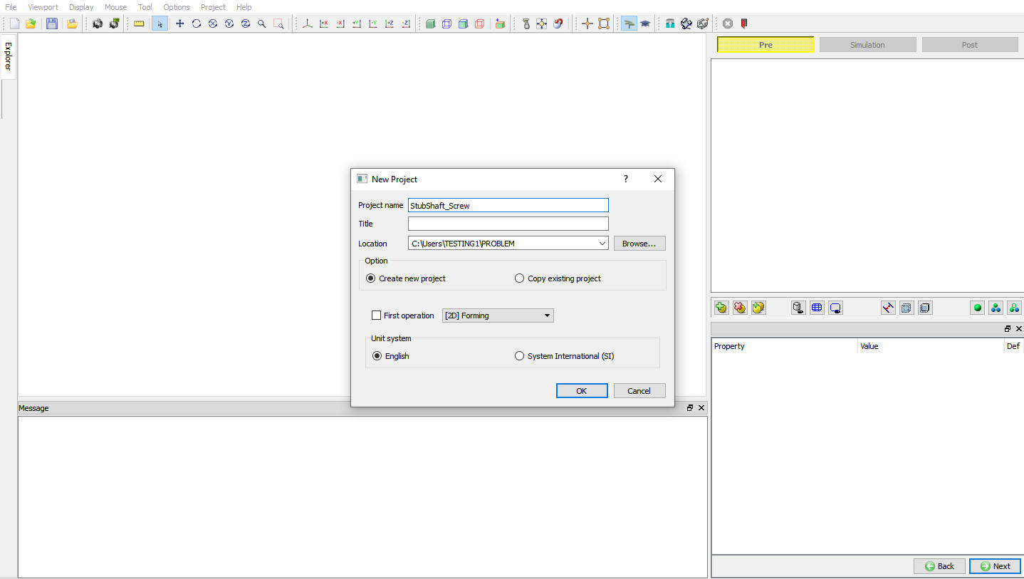
MO wizard will open along with project naming window (see Fig. L25.62.). In the field of project name, in this session we use ‘**StubShaft_Screw** ’ as the project name. Click on ![]() to continue to open the operation.
to continue to open the operation.
Problem defining window
Add Forming Operation
Add 2D Forming operation from the Explorer Operations list. Add the operation by clicking on ![]() button or user can also add by drag and drop into the Operation Editor.
button or user can also add by drag and drop into the Operation Editor.
Importing the DB
After adding 2D Forming operation, import previously simulated Stub_shaft_Warm.DB , select the f**irs t step of the third operation** and click on ![]() .
.
Punch Definition
Punch Movement Definition
Select the movement type as Screw press.
Specify:
Energy = 9 Klb-in
Moment of inertia = 0.125 Klb-in-s^2
Lead Screw Pitch = 5 in/rev
Efficiency = 0.8
We will keep rest of the settings as imported. click on ![]() until DB Generation page.
until DB Generation page.
Generate DB
Check the data and generate the DB. After generating DB switch to ![]() mode to run the simulation.
mode to run the simulation.
Running simulation
Click on the ![]() action label to open the Run Options. Use the default Continue Run option to select “Continue from the last step ” option and then select the Simulation mode as Interactive and click on
action label to open the Run Options. Use the default Continue Run option to select “Continue from the last step ” option and then select the Simulation mode as Interactive and click on ![]() button to run the simulation.
button to run the simulation.
After simulation complete, switch to ![]() tab.
tab.
Post processor
In Step Browser click on ![]() button to view all steps. Play through the steps to see the deformation.
button to view all steps. Play through the steps to see the deformation.
Go to the load-stroke plot and plot the punch velocity vs time. Plot the load vs. time.
User can rerun the simulation from the beginning with a higher energy.
Warm Stub shaft with Hammer movement
Opening project file
On a Windows machine , go to the ![]() button select DEFORM-v1x.xxx (.xxx indicates version number E.g. v14.0.2) and select DEFORM GUI Main vxx.xx from the menu. The DEFORM GUI Main window will appear.
button select DEFORM-v1x.xxx (.xxx indicates version number E.g. v14.0.2) and select DEFORM GUI Main vxx.xx from the menu. The DEFORM GUI Main window will appear.
Create a new problem either by selecting File![]() New Problem or by clicking the New Problem
New Problem or by clicking the New Problem ![]() icon. The Problem Setup window will appear. Select “ Integrated Manufacturing Process “ radio button and unit system as “English “ using radio button. Define Problem Name as “StubShaft_Hammer “ and make sure the “Show option dialog ” check box is turned on (if we do not turn on the “Show option dialog” check box, then we will not get the New Project dialog). Then click on
icon. The Problem Setup window will appear. Select “ Integrated Manufacturing Process “ radio button and unit system as “English “ using radio button. Define Problem Name as “StubShaft_Hammer “ and make sure the “Show option dialog ” check box is turned on (if we do not turn on the “Show option dialog” check box, then we will not get the New Project dialog). Then click on ![]() button to open a new problem using the Deform Integrated Manufacturing Process.
button to open a new problem using the Deform Integrated Manufacturing Process.
MO wizard will open along with project naming window (see Fig. L25.63.). In the field of project name, in this session we use ‘**StubShaft_Hammer** ’ as the project name. Click on ![]() to continue to open the operation.
to continue to open the operation.

Problem defining window
Add Multi Blow Forging Operation
Add 2D Multi Blow Forging operation from the Explorer Operations list. Add the operation by clicking on ![]() button or user can also add by drag and drop into the Operation Editor.
button or user can also add by drag and drop into the Operation Editor.
Importing the DB
After adding 2D Multi Blow Forging operation, import previously simulated Stub_shaft_Warm.DB , select the first step of the third operation and click ![]() .
.
Punch Definition
Punch Movement Definition
Select the movement type as Hammer.
Specify Hammer controls.
Set:
Energy = 6 Klb-in
Mass = 0.03 Klb-s^2/in
Blow table
In the Blow table page, set 0.5 for the efficiency and define the number of hits as 4.
We will keep rest of the settings as imported. click on ![]() until DB Generation page.
until DB Generation page.
Generate DB
Check the data and generate the DB. After generating DB switch to ![]() mode to run the simulation.
mode to run the simulation.
Note : While running the simulation, if the stopping criteria is met then further operations will not simulated.
Running simulation
Click on the ![]() action label to open the Run Options. Use the default Continue Run option to select “Continue from the last step ” option and then select the Simulation mode as Interactive and click on
action label to open the Run Options. Use the default Continue Run option to select “Continue from the last step ” option and then select the Simulation mode as Interactive and click on ![]() button to run the simulation. As we click on
button to run the simulation. As we click on ![]() button simulation starts.
button simulation starts.
After simulation complete, switch to ![]() tab.
tab.
Post processor
In Step Browser click on ![]() button to view all steps. Play through the steps to see the deformation.
button to view all steps. Play through the steps to see the deformation.
Go to the load-stroke plot and plot the punch velocity vs time. Plot the load vs. time.
User can rerun the simulation from the beginning with a higher energy.