2D Inverse Heat Lab1
Problem Summary:
This lab will demonstrate how to use the Inverse Heat Transfer Wizard to determine heat transfer coefficients between workpiece and media during a heat transfer process. Temperature measurement data is needed. Heat transfer coefficients can be function of temperature or time. Multiple zones of heat-transfer coefficients are assigned to the workpiece.
1.1. Starting a new problem
1.2. Set Geometry type and mode
1.3. Setting Process Conditions
1.4. Defining Material
1.5. Defining Workpiece Object
1.6. Import geometry
1.7. Generate mesh
1.8. Assigning Material
1.9. Generating Structured Mesh
1.10. BCC Definition
1.11. Temperature Measurement Points
1.12. Defining Time Zones
1.13. HT Zone Partitioning
1.14. Defining Heat Transfer Zones
1.15. Defining Step controls
1.16. Optimization control
1.17. Database Generation
1.18. Optimization
1.19. Optimization results
Starting a new problem
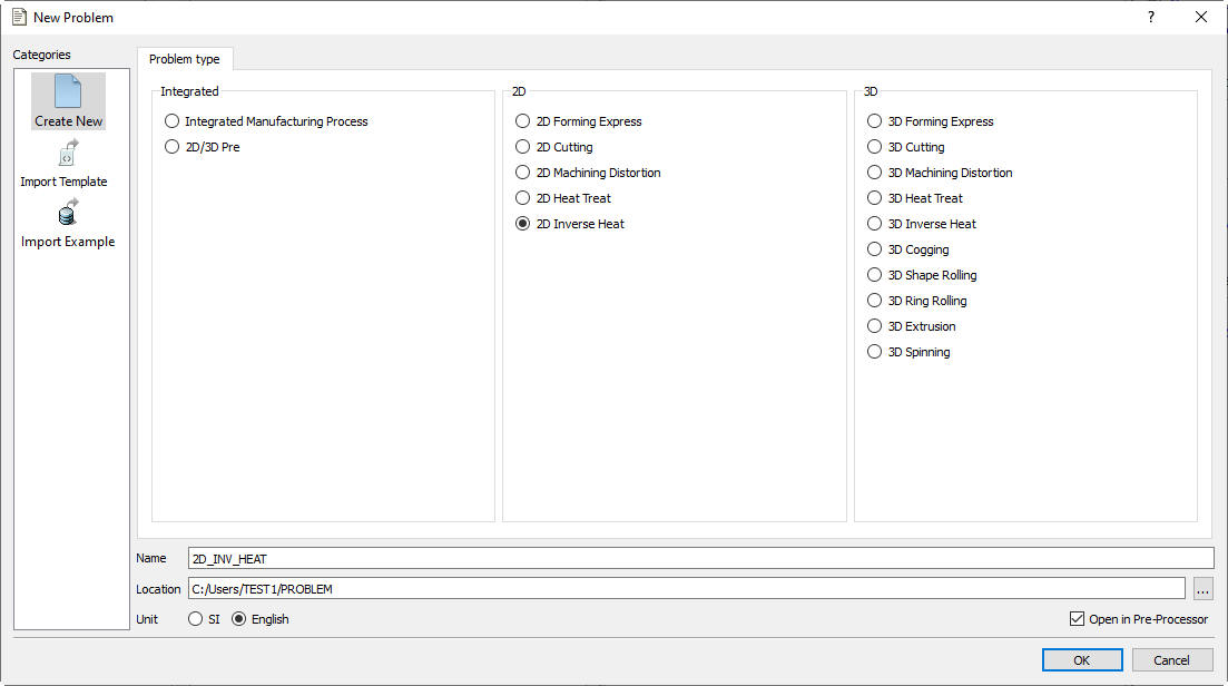
Start a new Inverse Heat Transfer Wizard problem with problem ID SIMPLE_INVHEAT. You can do so by clicking the ![]() button and choose “2D Inverse Heat ”, enter Problem name as “SIMPLE_INVHEAT “ and choose “English ” for “Unit System” (see Fig. 2DINVL1.1.). You can select the directory under Location field and then click
button and choose “2D Inverse Heat ”, enter Problem name as “SIMPLE_INVHEAT “ and choose “English ” for “Unit System” (see Fig. 2DINVL1.1.). You can select the directory under Location field and then click ![]() on to open Inverse Heat wizard.
on to open Inverse Heat wizard.
Problem Setup window
Set Geometry type and mode
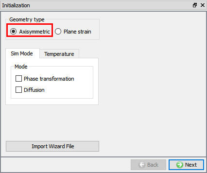
As the 2D Inverse Heat wizard opens, you should see a window as shown in Fig. 2DINVL1.2. Set “GeometryType ” as “Axisymmetric ”. If user is interested in calculating transformations or atom content due to diffusion then user can turn on respective check boxes under “Mode ” tab. In this lab we will not turn on any check box as we will be calculating only heat transfer co-efficients. Click on ![]() .
.
Initialization Window
Setting Process Conditions
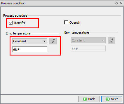
In this page user can set the environment conditions. If the process involves Quenching and heat transfer then respective check boxes can be turned on to define the environment conditions. Our process involves only heat transfer and environment temperature is constant, hence turn on “Transfer ” check box and define environment temperature as 68°F (see Fig. 2DINVL1.3.). Click on ![]() .
.
Setting up Process conditions
Defining Material
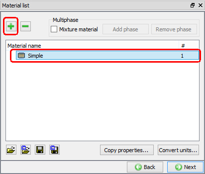
In page “Material list”, click on ![]() button to create a new material and rename the material to “Simple ” by clicking on the added “New Material” (see Fig. 2DINVL1.4.). Click on
button to create a new material and rename the material to “Simple ” by clicking on the added “New Material” (see Fig. 2DINVL1.4.). Click on ![]() to define material properties.
to define material properties.
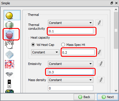
Select Thermal tab and enter0.1 for ThermalConductivity , 0.2 for HeatCapacity , and 0.3 for Emissivity as constant values as shown in Fig. 2DINVL1.5. Click on ![]() until “Workpiece” page.
until “Workpiece” page.
Creating New Material
Defining Thermal Material properties
Defining Workpiece Object
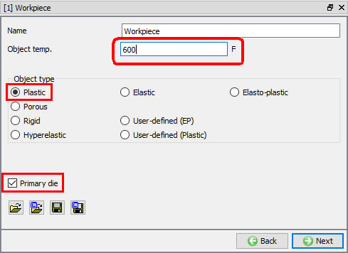
In workpiece page define Object Temp. as 600 °F as shown in Fig. 2DINVL1.6. Make sure the object type is Plastic and Primary Die check box is checked. Click on ![]() to geometry page.
to geometry page.
Workpiece Object Definition
Import geometry
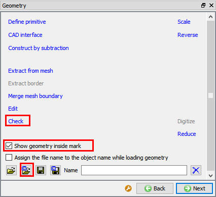
In “Geometry” page, click on ![]() icon and import geometry file “SIMPLE_INVHEAT.IGS ” from ‘/2D/LABS’ directory as shown in Fig. 2DINVL1.7.By default “Show geometry inside mark” check box will be Turned on if not Turned on the check box and click on
icon and import geometry file “SIMPLE_INVHEAT.IGS ” from ‘/2D/LABS’ directory as shown in Fig. 2DINVL1.7.By default “Show geometry inside mark” check box will be Turned on if not Turned on the check box and click on ![]() label to check and correct the geometry, see Fig. 2DINVL1.7.
label to check and correct the geometry, see Fig. 2DINVL1.7.
Geometry window
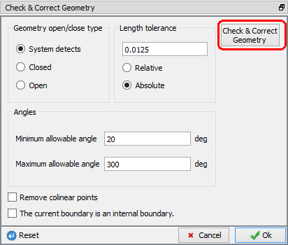
Click on ![]() and then click
and then click ![]() button to geometry correction pop-up and then click on
button to geometry correction pop-up and then click on ![]() button to come out of Geometry Correction page, see Fig. 2DINVL1.8. Click on
button to come out of Geometry Correction page, see Fig. 2DINVL1.8. Click on ![]() to mesh page.
to mesh page.
Check and Correct Geometry window
Generate mesh
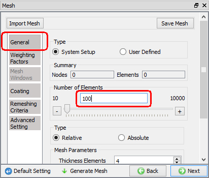
While user is in “Mesh” page, expert mode can be used to access the advanced mesh options. Click on ![]() icon in tool bar to change to expert mode and then enter 100 as target number of elements in “General ” tab for unstructured mesh, see Fig. 2DINVL1.9. Click on
icon in tool bar to change to expert mode and then enter 100 as target number of elements in “General ” tab for unstructured mesh, see Fig. 2DINVL1.9. Click on ![]() button. Click on
button. Click on ![]() to Material page to assign material.
to Material page to assign material.
Defining unstructured mesh
Assigning Material
Select material “Simple ” from the material list to assign to workpiece as shown in Fig. 2DINVL1.10.
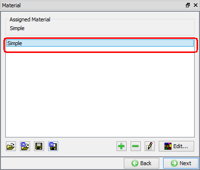
Assigning Material
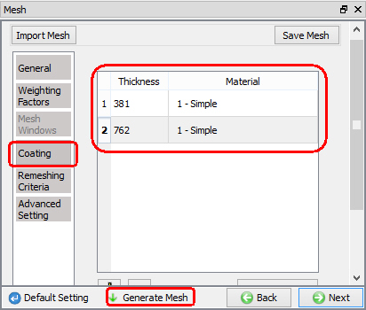
Generating Structured Mesh
The structured surface mesh helps provide better thermal solution accuracy with less computing time. Hence click ![]() from Material page. We will use 2 layers of structured surface mesh using coating mesh with thickness of 381Microns and 762microns for layer 1 and 2 respectively with “Simple ” material and click on
from Material page. We will use 2 layers of structured surface mesh using coating mesh with thickness of 381Microns and 762microns for layer 1 and 2 respectively with “Simple ” material and click on ![]() button as shown in Fig. 2DINVL1.11. Do not use “Generate Coating” button. Click
button as shown in Fig. 2DINVL1.11. Do not use “Generate Coating” button. Click ![]() button for the pop-up “Do you want generate coating mesh?”. After generating mesh Zoom into the top right corner and check generated mesh for structured layers. Meshed object looks as shown in Fig. 2DINVL1.12. Click on
button for the pop-up “Do you want generate coating mesh?”. After generating mesh Zoom into the top right corner and check generated mesh for structured layers. Meshed object looks as shown in Fig. 2DINVL1.12. Click on ![]() until BCC page.
until BCC page.
Structured mesh generation using Coating mesh
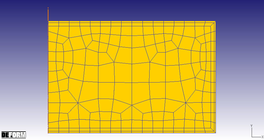
Meshed Workpiece After Generating Structured Mesh
BCC Definition
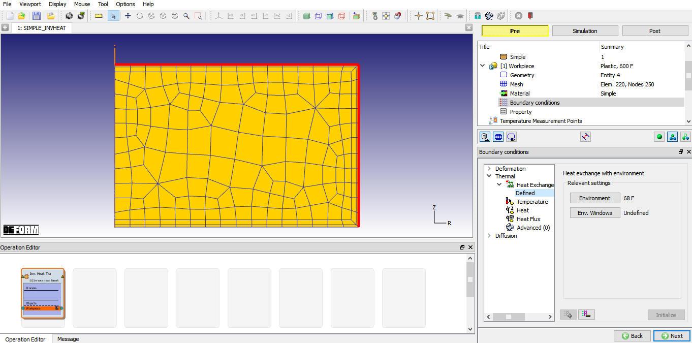
By default “Heat Exchange with Environment” BCC and Axi-symmetric BCC (Vx = 0) are assigned to workpiece and these can be verified by selecting the respective BCC from the BCC tree. Select “Defined” under “Heat Exchange with Environment” BCC and then click ![]() on button to delete default BCC. Now to define “Heat Exchange with Environment” BCC, select right edge and top edge of the workpiece and then click on
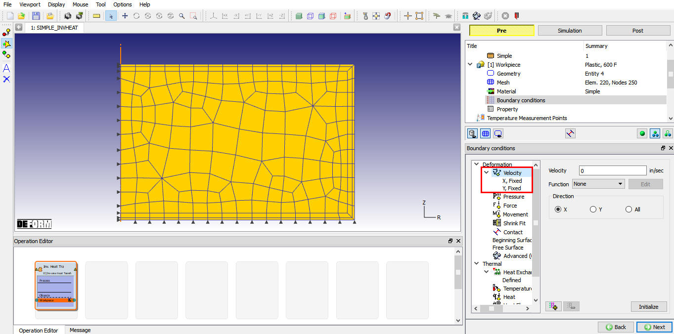
on button to delete default BCC. Now to define “Heat Exchange with Environment” BCC, select right edge and top edge of the workpiece and then click on ![]() button, assigned BCC are as shown in Fig. 2DINVL1.13. To define Symmetry on bottom edge select “Velocity” under “Deformation” BCC, then select direction as Y, make sure velocity value is zero and then select bottom edge and then click on
button, assigned BCC are as shown in Fig. 2DINVL1.13. To define Symmetry on bottom edge select “Velocity” under “Deformation” BCC, then select direction as Y, make sure velocity value is zero and then select bottom edge and then click on ![]() button, defined BCC are as shown in Fig. 2DINVL1.14. Click on
button, defined BCC are as shown in Fig. 2DINVL1.14. Click on ![]() until “Temperature Measurement Points” page.
until “Temperature Measurement Points” page.
Defined Heat Exchange with Environment BCC
Defined Symmetry Bcc
Temperature Measurement Points
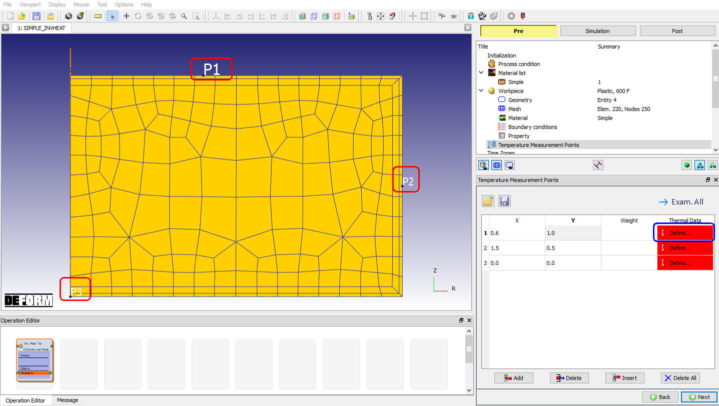
In “Temperature Measurement Points” page, click ![]() button three times and input coordinates (0.6, 1.0), (1.5, 0.5), and (0.0, 0.0) in the table for point 1, 2, and 3, respectively as shown in Fig. 2DINVL1.15. Thermal history data for each point can be defined by clicking on the
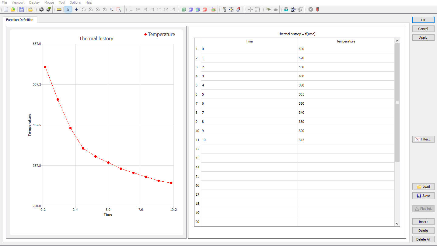
button three times and input coordinates (0.6, 1.0), (1.5, 0.5), and (0.0, 0.0) in the table for point 1, 2, and 3, respectively as shown in Fig. 2DINVL1.15. Thermal history data for each point can be defined by clicking on the ![]() button in the last column of the table. Click on Load and load “SIMPLE_INVHEAT_P1_Thermal_History.DAT” file for point 1 from the /Labs folder and click button (see Fig. 2DINVL1.16.), similarly load SIMPLE_INVHEAT_P2_Thermal_History.DAT and SIMPLE_INVHEAT_P3_Thermal_History.DAT for point 2 and 3 respectively. “Define” button in the last column of the table will change into
button in the last column of the table. Click on Load and load “SIMPLE_INVHEAT_P1_Thermal_History.DAT” file for point 1 from the /Labs folder and click button (see Fig. 2DINVL1.16.), similarly load SIMPLE_INVHEAT_P2_Thermal_History.DAT and SIMPLE_INVHEAT_P3_Thermal_History.DAT for point 2 and 3 respectively. “Define” button in the last column of the table will change into ![]() after you had defined the Thermal History Data for the point. Click on
after you had defined the Thermal History Data for the point. Click on ![]() .
.
Temperature measurement Points page
Thermal History Data window for Point 1
Defining Time Zones
In time zones page user can define time zones for Quenching and Transfer. Since in this lab we had opted to simulate only transfer, only Transfer time zone definition is available. We would like to simulate the process for 10 sec as the last point of temperature measurement is available from thermal history is at 10 sec. So enter Start time as 0sec and End time as 10 sec. Thermal History graph of all the points within the specified time can be seen in display area, see Fig. 2DINVL1.17. Click on ![]() .
.
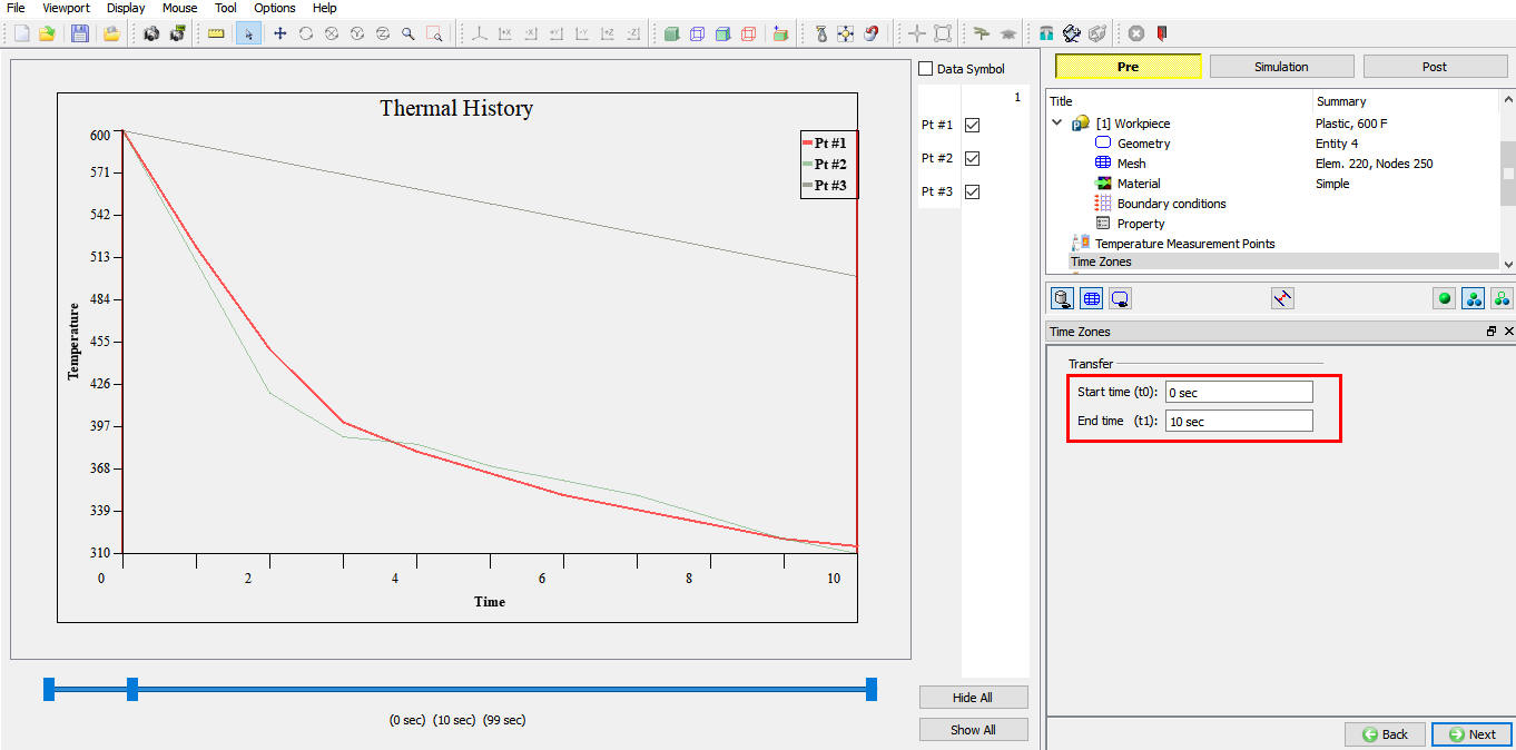
Transfer Time Definition in Time Zone page
HT Zone Partitioning
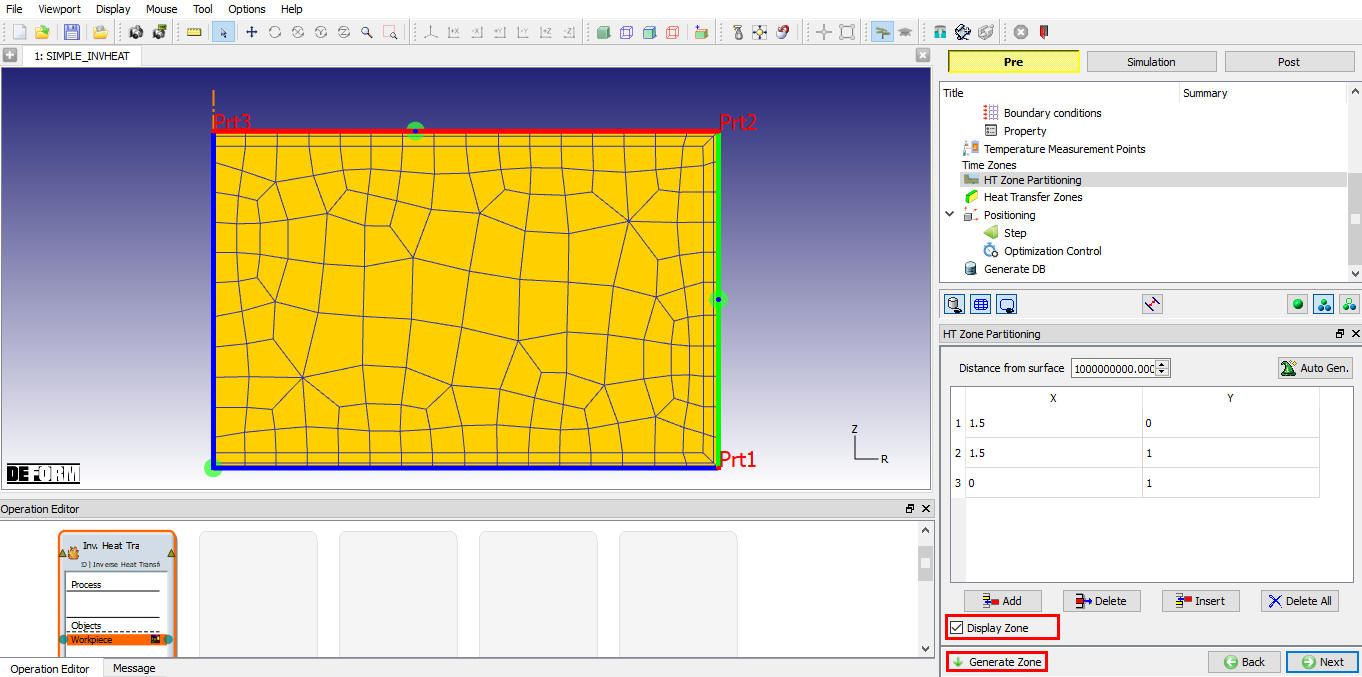
In page “HT Zone Partioning” we can see that system has automatically generated zones based upon temperature points defined, Turn on “Display Zone” check box to verify the zones created. We can see that these zones are created without considering the symmetry on bottom edge and also the zones start and end points are on the edges hence we will redefine the partitioning so that we can delete unwanted zones. We will delete the already defined zones using “Delete All” button. By default entire outer surface edges will be considered as one zone. After deleting points, we will select three points in anti-clock wise, bottom right corner, top right corner and top left corner as shown in Fig. 2DINVL1.18. Click on ![]() to generate zones. Zones are created between the pair of points selected, see Fig. 2DINVL1.18. Click on
to generate zones. Zones are created between the pair of points selected, see Fig. 2DINVL1.18. Click on ![]() .
.
HT Zone Partitioning window
Defining Heat Transfer Zones
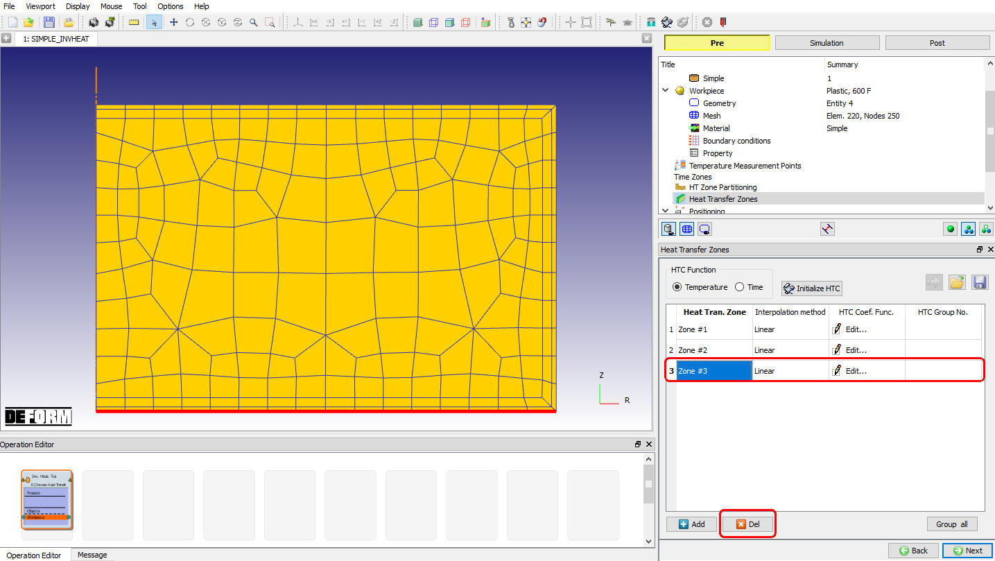
In “Heat Transfer Zones” page, we can see that 3 zones are created, Zone #1 covering the right edge, Zone #2 covering the Top edge and Zone #3 covering the bottom symmetry edge. We do not require Zone #3, hence select Zone #3 and click on ![]() button as shown in Fig. 2DINVL1.19.
button as shown in Fig. 2DINVL1.19.
Deleting Unwanted Zone #3
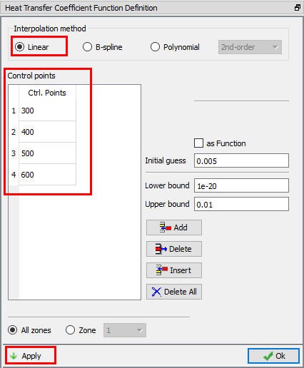
After deleting unwanted Zone #3, click on ![]() button to define control points and limits, make sure HTC function is based on temperature. By default system will add some control points, we will delete them for this lab and use four points. Click on
button to define control points and limits, make sure HTC function is based on temperature. By default system will add some control points, we will delete them for this lab and use four points. Click on ![]() button and delete all rows except 4 rows and then enter four values 300 , 400 , 500 and 600 , see Fig. 2DINVL1.20. Make sure interpolation method is Linear and initial guess, lower and upper bounds are fine. Click on
button and delete all rows except 4 rows and then enter four values 300 , 400 , 500 and 600 , see Fig. 2DINVL1.20. Make sure interpolation method is Linear and initial guess, lower and upper bounds are fine. Click on![]() button, Click
button, Click ![]() to close Initializing Window.
to close Initializing Window.
Deleting Unwanted Zone #3
Control points and limits settings can be set for each zone separately using ![]() button next Zone in “Heat Transfer Zones” page, see Fig. 2DINVL1.20. Click on
button next Zone in “Heat Transfer Zones” page, see Fig. 2DINVL1.20. Click on ![]() until “Step” page.
until “Step” page.
Defining Step controls
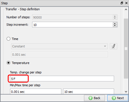
In “Step” page, change “Temperature change per step” to 5.0 and leave other values to defaults as shown in Fig. 2DINVL1. 21. Click on ![]() .
.
Defining Step controls
Optimization control
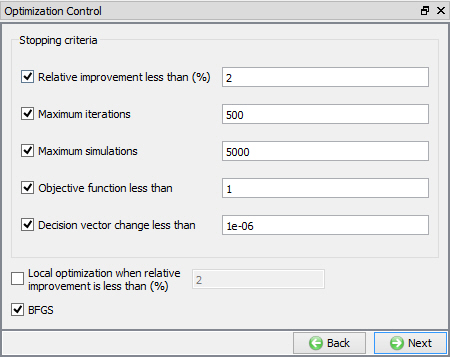
In “Optimization Control” page as shown in Fig. 2DINVL1.22., all default settings are fine, so click on ![]() .
.
Optimization control window
Database Generation
In DB Generation page click on ![]() to verify the set up for errors and warnings, you should see a message “Data Valid!” if there are no errors. Click on
to verify the set up for errors and warnings, you should see a message “Data Valid!” if there are no errors. Click on ![]() to generate Database.
to generate Database.
Optimization
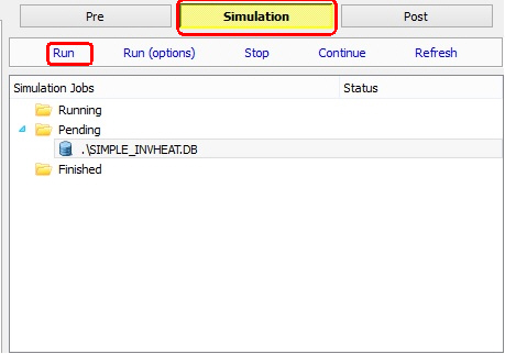
After Database is generated switch to ![]() tab above the object tree and click on
tab above the object tree and click on ![]() to start the optimization, see Fig. 2DINVL1.23. You can see a message “MULTIPLE OPERATION COMPLETED.” at the end of Simulation Log file after optimization is completed.
to start the optimization, see Fig. 2DINVL1.23. You can see a message “MULTIPLE OPERATION COMPLETED.” at the end of Simulation Log file after optimization is completed.
Running Optimization
Optimization results
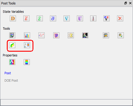
To view optimization results switch to Post mode by clicking on ![]() tab. In Tools” page under “Tools” you can see two icons (see Fig. 2DINVL1.24.),
tab. In Tools” page under “Tools” you can see two icons (see Fig. 2DINVL1.24.),
![]()
![]() To view Optimized HTC values.
To view Optimized HTC values.
![]()
![]() To view simulated temperature values at Temperature Measurement Points.
To view simulated temperature values at Temperature Measurement Points.
Post Tools to view Optimization Results
Click on ![]() to view optimized HTC values for each zone, a Heat Transfer Zone window will open as shown in Fig. 2DINVL1.25. Select each zone and click on
to view optimized HTC values for each zone, a Heat Transfer Zone window will open as shown in Fig. 2DINVL1.25. Select each zone and click on ![]() to view optimized HTC values, see Fig. 2DINVL1.26. for Zone #1 optimized HTC values.
to view optimized HTC values, see Fig. 2DINVL1.26. for Zone #1 optimized HTC values.
![]() can be used to view objective value history, see Fig. 2DINVL1.27.
can be used to view objective value history, see Fig. 2DINVL1.27.
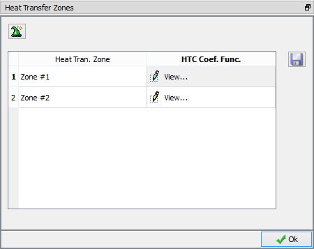
Heat Transfer Zones Window in Post Tab
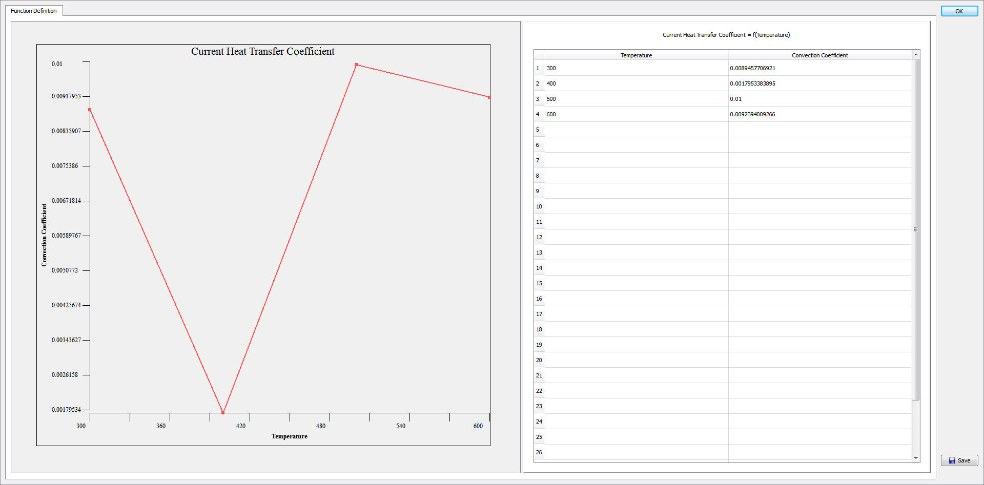
Optimized HTC values for Zone #1
Objective Value History
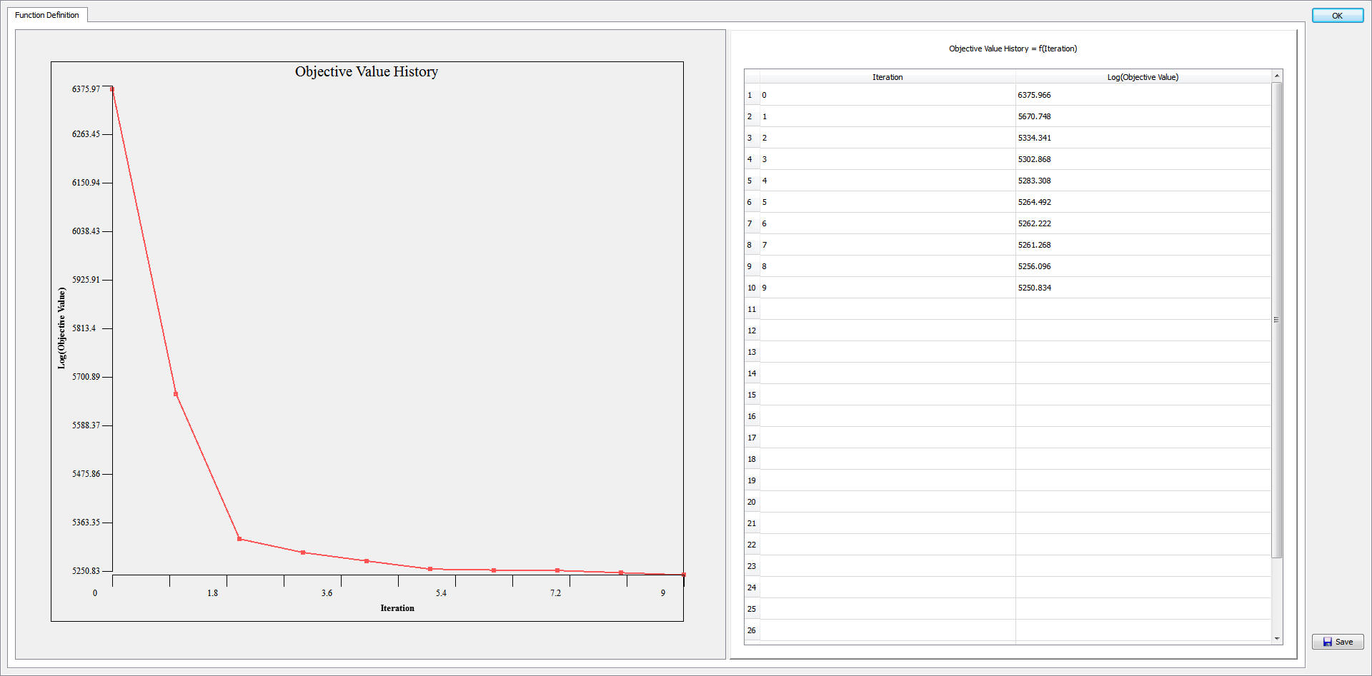
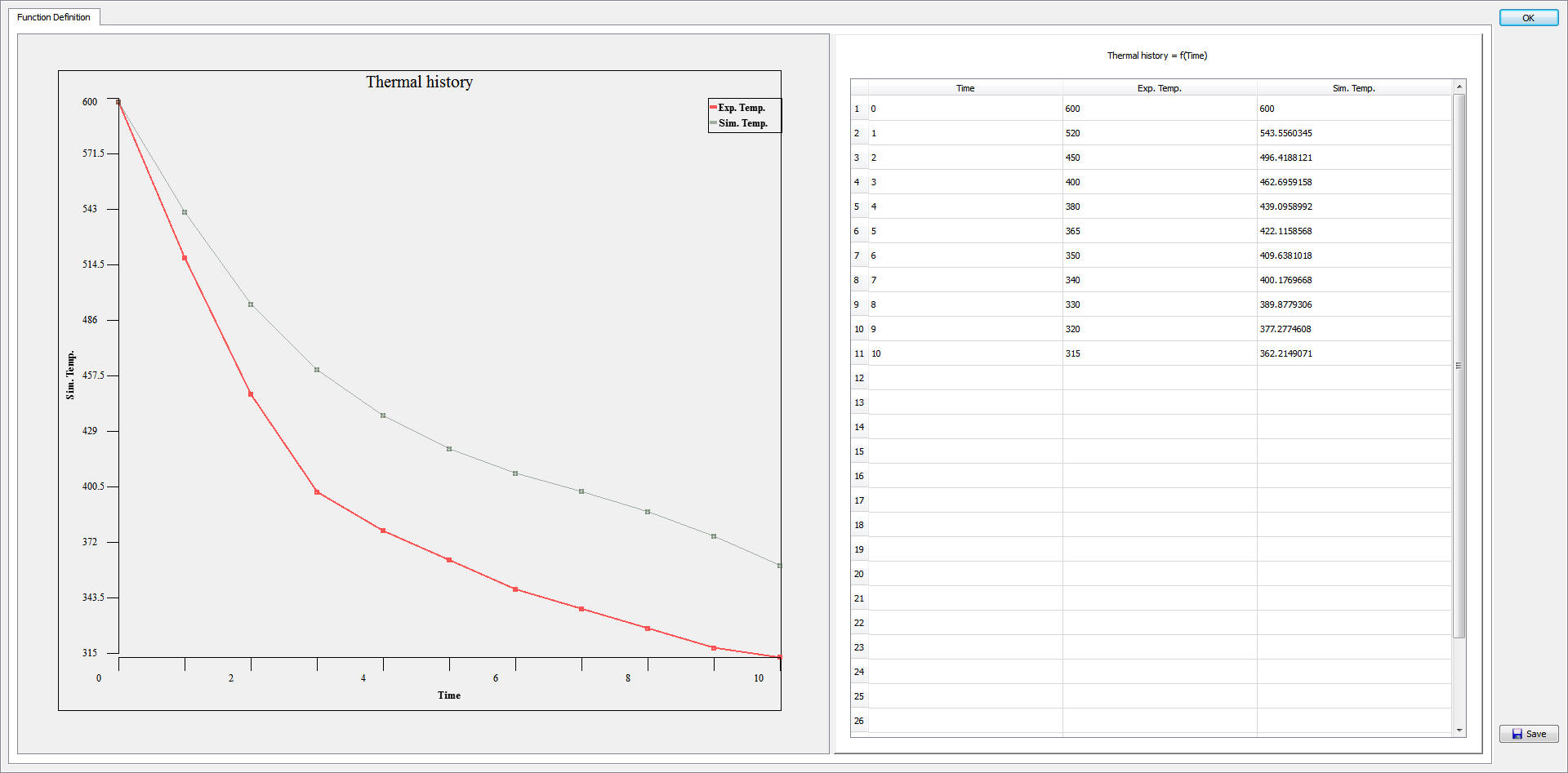
The local objective optimization result can be viewed using ![]() , it gives the comparison between the experimental temperature and the simulated temperature values when the optimized heat transfer coefficient values are used. These values can be saved if necessary using
, it gives the comparison between the experimental temperature and the simulated temperature values when the optimized heat transfer coefficient values are used. These values can be saved if necessary using ![]() button (see Fig. 2DINVL1.28.). User can select a point (See Figure 28) and click on
button (see Fig. 2DINVL1.28.). User can select a point (See Figure 28) and click on ![]() to plot the comparison between the experimental temperature and the simulated temperature values or
to plot the comparison between the experimental temperature and the simulated temperature values or ![]() to plot for all values, Fig. 2DINVL1.29. shows the comparison between the experimental temperature and the simulated temperature values for Point 1.
to plot for all values, Fig. 2DINVL1.29. shows the comparison between the experimental temperature and the simulated temperature values for Point 1.
Temperature Measurement Points in Post
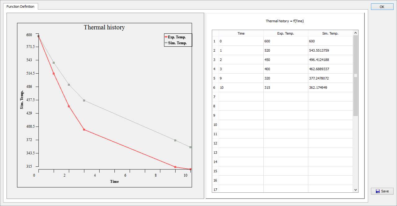
Local Objective Optimization Result for Point 1