Diffusion Bonding Lab1
1.1. Problem Summary
1.2. Build diffusion bonding model in DEFORM based on experimental data
1.3. FEM simulation of diffusion bonding process in DEFORM
1.3.1. Creating a New problem
1.3.2. Define simulation modes
1.3.3. Import Material
1.3.4. Add objects
1.3.5. Define Top Sheet
1.3.6. Define Bottom Sheet
1.3.7. Position the Sheets
1.3.8. Define Inter-object contacts
1.3.9. Define Boundary conditions for top and bottom sheet
1.3.10. Activate Diffusion Bonding
1.3.11. Define Diffusion bonding material data
1.3.12. Define Simulation step controls
1.3.13. Run the Simulation
1.3.14. Post Processing
Problem Summary
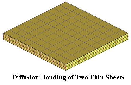
Diffusion bonding (DB) is a well-established technology for the manufacture of components from titanium alloy thin sheets. Time to achieve complete bonding is a function of temperature, pressure, and surface roughness. In this lab, the diffusion bonding of two thin sheets of titanium alloy (Ti-6Al-4V) at elevated temperature (1400F) under a 2-step pressure will be simulated.
The key points in this lab include:
-
Building diffusion bonding model in DEFORM based on artificial made up experimental data
-
Activation of diffusion bonding calculation in FEM model setup
-
Definition of 1% and 99% complete time for diffusion bonding as a function of temperature and pressure
-
Examination of the diffusion bonding percent at a selected step in the post processor
Build diffusion bonding model in DEFORM based on experimental data
The artificial made up experimental data for diffusion bonding between the couple of titanium alloy Ti-6Al-4V is given in Table 1. The data are not real experimental data, and are tuned only for demonstration purpose. As can be seen, for the same bonding time, the higher the temperature and the higher the pressure, the higher the bonding percent.
| Temperature (F) | Pressure (Ksi) | Time (hour) | Bond percent |
|---|---|---|---|
| 1400 | 0.145 | 1 | 0.12 |
| 0.145 | 3 | 0.197 | |
| 0.435 | 1 | 0.392 | |
| 0.435 | 3 | 0.726 | |
| 1500 | 0.145 | 1 | 0.612 |
| 0.145 | 2 | 0.928 | |
| 0.435 | 0.5 | 0.54 | |
| 0.435 | 1 | 0.835 |
Diffusion bonding data for the couple of a titanium alloy
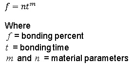
The surface roughness is assumed to be identical for all cases, and is not explicitly considered in DEFORM DB model. Under constant temperature and pressure, the relation between bonding percent and time in DEFORM is described by the equation,
 | EQ(1)
—|—
For each DB condition with a constant temperature and pressure, by fitting bonding percent versus time, the values of m andn can be determined. Then the time for 1% bonding and the time for 99% bonding can be determined according to Equation (1). The results are summarized in Table 2. The time for 1% bonding and the time for 99% bonding at different temperature and pressure are used to define the diffusion bonding model in DEFORM.
| Temperature (F) | Pressure (Ksi) | m | n | 1% bonding time (seconds) | 99% bonding time (seconds) |
|---|---|---|---|---|---|
| 1400 | 0.145 | 0.451216 | 0.002982 | 14.6079 | 386701.8 |
| 0.435 | 0.56097 | 0.003966 | 5.2008 | 18773.32 | |
| 1500 | 0.145 | 0.600593 | 0.004476 | 3.8135 | 8018.60 |
| 0.435 | 0.628817 | 0.004846 | 3.1642 | 4719.57 |
Material parameters for diffusion bonding model
FEM simulation of diffusion bonding process in DEFORM
Creating a New problem
Create a new problem either by selecting File![]() **New Problem** or by clicking the New Problem
**New Problem** or by clicking the New Problem ![]() icon. The Problem Setup window will appear. Select “ Integrated Manufacturing Process “ radio button and unit system as “English “ radio button in unit field. Define Problem Name as “ DiffusionBonding “ and make sure the “Show option dialog” check box is turned on (if we do not turn on the “Show option dialog ” check box, then we will not get the New Project dialog in MO UI). Then click on
icon. The Problem Setup window will appear. Select “ Integrated Manufacturing Process “ radio button and unit system as “English “ radio button in unit field. Define Problem Name as “ DiffusionBonding “ and make sure the “Show option dialog” check box is turned on (if we do not turn on the “Show option dialog ” check box, then we will not get the New Project dialog in MO UI). Then click on ![]() button to open a new Problem using the Deform Integrated Manufacturing Process.
button to open a new Problem using the Deform Integrated Manufacturing Process.
Multiple operation wizard will open with the New Project dialog as shown in Fig. DBL1.1., at this point user will be prompted to specify a project name (system will create a separate folder with this project name) and title for this session. In this lab we use ‘DiffusionBonding ” as the project name. Select First operation as 3DForming and keep the unit system as English , Click ![]() .
.
Added 3D Forming operation into Operation Editor
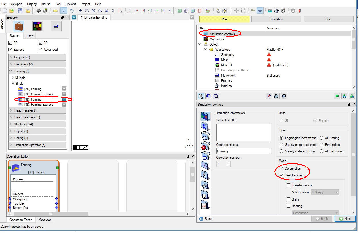
Define simulation modes
This will be demonstrated in expert mode so select the Expert mode ![]() icon in the tool bar. In simulation controls page set the simulation modes by checking Deformation and HeatTransfer(See Fig. DBL1.1.). Click
icon in the tool bar. In simulation controls page set the simulation modes by checking Deformation and HeatTransfer(See Fig. DBL1.1.). Click ![]() to import the material.
to import the material.
Import Material
In Material page click on the ![]() icon “Load Material data from Library” to import material Titanium alloy Ti-6Al-4V from DEFORM material library. Click
icon “Load Material data from Library” to import material Titanium alloy Ti-6Al-4V from DEFORM material library. Click ![]() until Objects page.
until Objects page.
Add objects
From the list, keep only two objects and delete the other object. (See Fig. DBL1.2.)
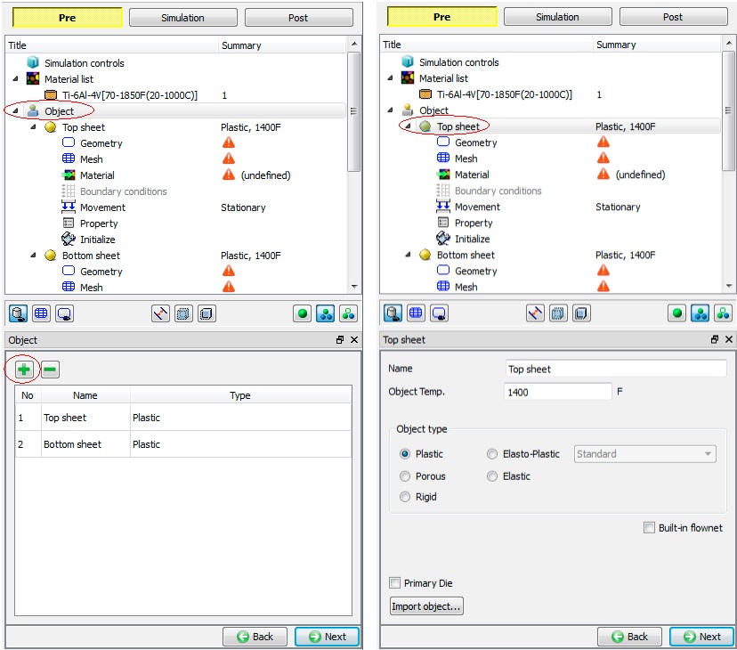
Object page and Top sheet general page
Define Top Sheet
Change the name of the first object to Topsheet , Set the object type as Plastic and object temperature to 1400 °F. Click ![]() to define the top sheet geometry. ( Fig. DBL1.2.)
to define the top sheet geometry. ( Fig. DBL1.2.)
In geometry page, click the ![]() button (See Fig. DBL1.3.). Select the “Box “ shape, and define the following box size: Width(W) = 5 inches, Height(H) = 0.2 inch, and Length(L) = 5 inches. Click the
button (See Fig. DBL1.3.). Select the “Box “ shape, and define the following box size: Width(W) = 5 inches, Height(H) = 0.2 inch, and Length(L) = 5 inches. Click the ![]() button to exit the window. The defined box appears in the display window.
button to exit the window. The defined box appears in the display window.

Define the geometry of top sheet
In order to generate the brick mesh, click the ![]() in the geometry page. Select the “Extrude “ radio button. In order to define the start surface and end surface to extrude during mesh generation, select the icon “Selection mode” (
in the geometry page. Select the “Extrude “ radio button. In order to define the start surface and end surface to extrude during mesh generation, select the icon “Selection mode” (![]() ) in the tool bar, select the Startsurface , then pick up a topsurface of the topsheet , and click the
) in the tool bar, select the Startsurface , then pick up a topsurface of the topsheet , and click the ![]() button in the window to accept the definition (See Fig. DBL1.4.). The existing definition can be removed by selecting it and clicking the button
button in the window to accept the definition (See Fig. DBL1.4.). The existing definition can be removed by selecting it and clicking the button ![]() . Similarly define the bottomsurface of the topsheet as Endsurface. Click the
. Similarly define the bottomsurface of the topsheet as Endsurface. Click the ![]() button to exit the brick mesh geometry setup. Click
button to exit the brick mesh geometry setup. Click ![]() to generate mesh.
to generate mesh.
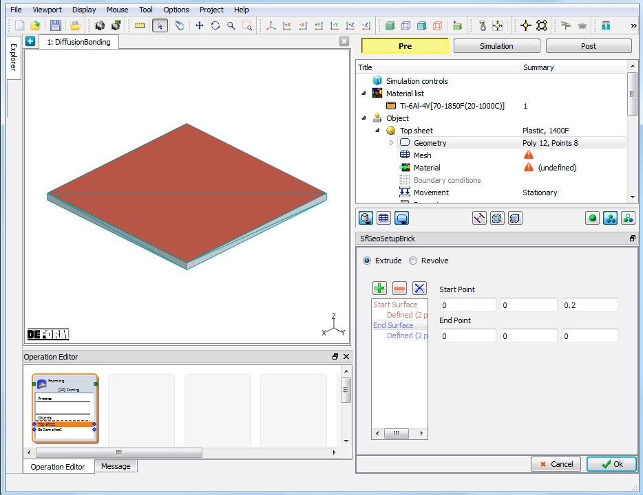
Define the start surface and end surface of brick mesh
In mesh page general tab select the “Brick Mesh “ radio button and the “Uniform thickness “ radio button, set the “# of layers “ to 4. In the “2D Cross Section “ tab check mapped mesh generation checkbox, set the targetnumberofelements to 100 , thickness elements to 10 and the sizeratio to 1. Click ![]() and click
and click ![]() for Default Boundary condition popup as we will be defining required BCC. As a result, 400 brick elements with 605 nodes will be generated (See Fig. DBL1.5.). Click
for Default Boundary condition popup as we will be defining required BCC. As a result, 400 brick elements with 605 nodes will be generated (See Fig. DBL1.5.). Click ![]() to assign material.
to assign material.
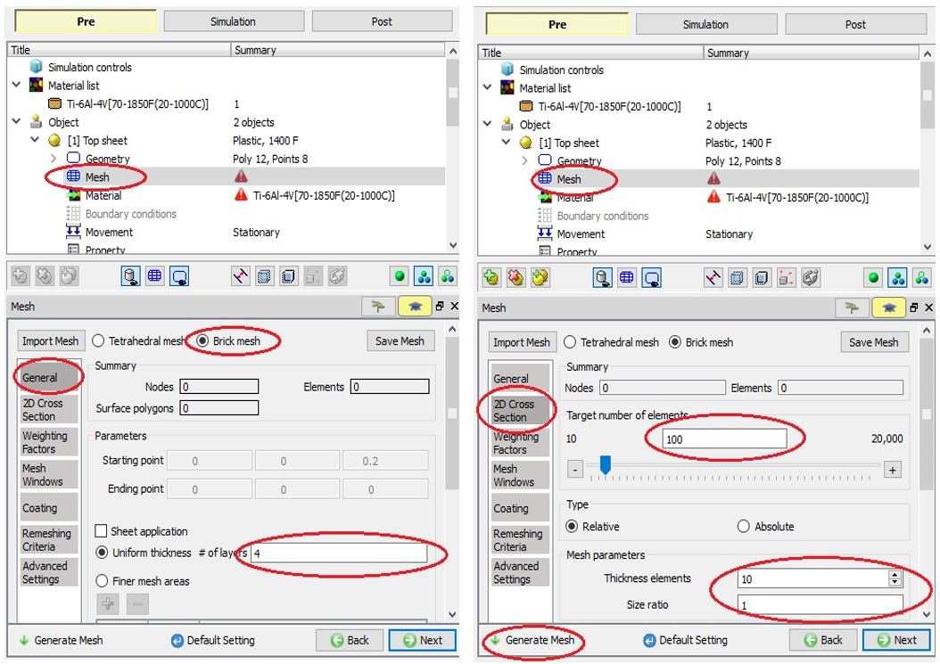
Brick mesh generation settings
In material page assign the material “Ti-6Al-4V “ to the top sheet by selecting the material in the object material page.
Define Bottom Sheet
Generate the bottom sheet box geometry with same dimension as top sheet and also generate the brick mesh similar to it.
Position the Sheets
In order to place the top sheet in the correct position with respect to the bottom sheet, click the Positioning branch in the operation tree; click the ![]() button, the “Object positioning” window opens (See Fig. DBL1.6.). Select the top sheet as the positioning object and the “Offset “ as the positioning method. Input the following displacement: X=0, Y=0, and Z=0.2. Click
button, the “Object positioning” window opens (See Fig. DBL1.6.). Select the top sheet as the positioning object and the “Offset “ as the positioning method. Input the following displacement: X=0, Y=0, and Z=0.2. Click ![]() . The top sheet is moved to the top of the bottom sheet. Click
. The top sheet is moved to the top of the bottom sheet. Click ![]() until Contact page to define inter-object contact.
until Contact page to define inter-object contact.
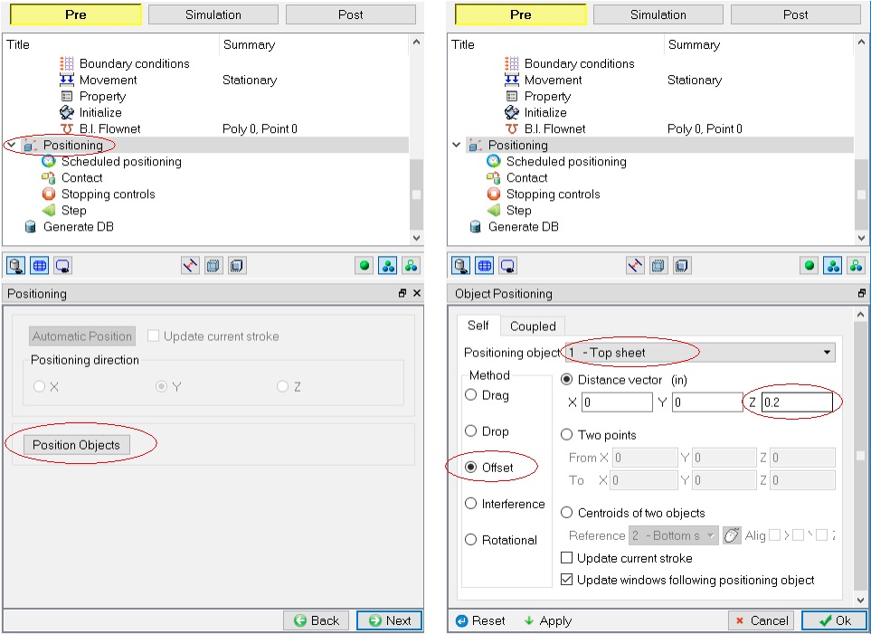
Positioning of top sheet
Define Inter-object contacts
In the contact page, click the button ![]() to add a new contact (See Fig. DBL1.7.). Select the bottomsheet as the “Master “ object and the topsheet as the “Slave “ object. Accept the other default setting. Click the
to add a new contact (See Fig. DBL1.7.). Select the bottomsheet as the “Master “ object and the topsheet as the “Slave “ object. Accept the other default setting. Click the ![]() button and then the
button and then the ![]() button to generate the contact conditions.
button to generate the contact conditions.
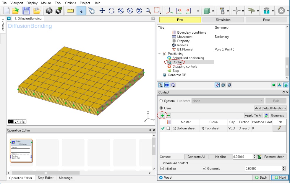
Define contact condition
Define Boundary conditions for top and bottom sheet
To remove the rigid movement of the objects, define the following zero velocity boundary conditions as shown in Fig. DBL1.8. For the plane with X= 2.5, Vx=0; for the plane with Y=2.5 , Vy=0; for the bottom surface of the bottom sheet, Vz=0.
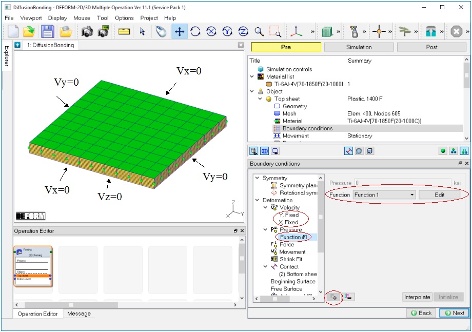
Define boundary conditions
In order to define the applied pressure for diffusion bonding process, click the top sheet Boundary conditions branch in the operation tree window (See Fig. DBL1.8.). In the popup “Boundary conditions “ window, select the branch ![]() . Select the data type as function and click the button
. Select the data type as function and click the button ![]() . In the popup window, define pressure data as a function of time, see Fig. DBL1.9. and Table 3. The applied pressure is 0.145 ksi during the first 3 hours and 0.4351 ksi during the subsequent 2 hours. These pressure data are generated only for demonstration purpose. Then select the icon “Selection mode” (
. In the popup window, define pressure data as a function of time, see Fig. DBL1.9. and Table 3. The applied pressure is 0.145 ksi during the first 3 hours and 0.4351 ksi during the subsequent 2 hours. These pressure data are generated only for demonstration purpose. Then select the icon “Selection mode” (![]() ) in the tool bar, and use the picking tools on the left to select the top surface of the top sheet. Click the
) in the tool bar, and use the picking tools on the left to select the top surface of the top sheet. Click the ![]() button to apply the setting. After that, the defined function number is inserted under the deformation bcc sub-branch
button to apply the setting. After that, the defined function number is inserted under the deformation bcc sub-branch ![]() .
.
| Time (s) | Pressure (ksi) |
|---|---|
| 0 | -0.145 |
| 10800 | -0.145 |
| 10801 | -0.4351 |
| 18000 | -0.4351 |
The applied pressure as function of time
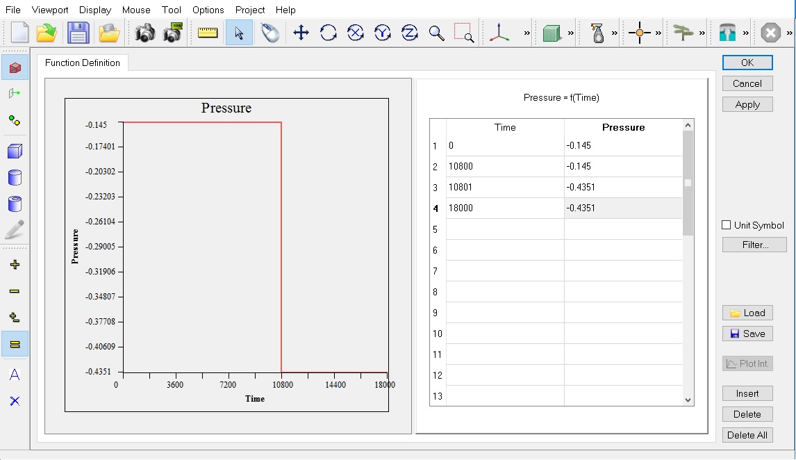
Define the applied pressure as a function of time
Activate Diffusion Bonding
In the operation tree window, click the Simulationcontrols branch. In the properties window, click the “Process condition “ icon (![]() ), and turn on the check box “Turn on diffusion calculation” (See Fig. DBL1.10.).
), and turn on the check box “Turn on diffusion calculation” (See Fig. DBL1.10.).
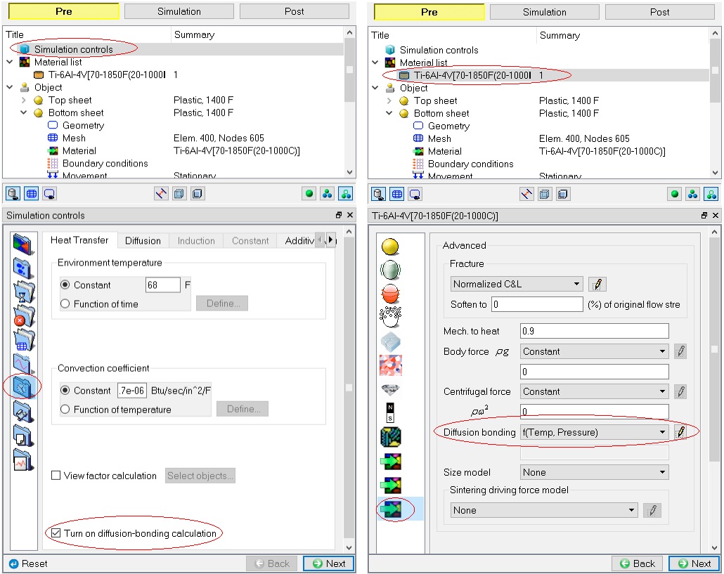
Turn on diffusion bonding calculation
Define Diffusion bonding material data
In the operation tree, select the material Ti-6Al-4V in the materiallist. In the properties window, select the ![]() page. Set the “Diffusion bonding “ data type as function of temperature and pressure , click the
page. Set the “Diffusion bonding “ data type as function of temperature and pressure , click the ![]() icon to edit the function data (See Fig. DBL1.11.). In the function data, there are two temperatures (1400F and 1500F) and two pressures (0.145 ksi and 0.4351 ksi). At each temperature and pressure, we define the 1% complete time and 99% complete time of diffusion bonding, with the unit of second, as calculated in Table 2 and shown in Fig. DBL1.11. These data are generated only for demonstration of this Lab.
icon to edit the function data (See Fig. DBL1.11.). In the function data, there are two temperatures (1400F and 1500F) and two pressures (0.145 ksi and 0.4351 ksi). At each temperature and pressure, we define the 1% complete time and 99% complete time of diffusion bonding, with the unit of second, as calculated in Table 2 and shown in Fig. DBL1.11. These data are generated only for demonstration of this Lab.
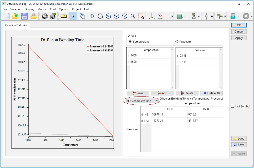
Define 1% complete time and 99% complete time for diffusion bonding
Define Simulation step controls
In the operation tree select the Step page, click on Guided mode ![]() , define the simulationsteps as 600 , stepincrement to save as 10 , the step increment is controlled by time , and the time increment for each step is 30 seconds. Click
, define the simulationsteps as 600 , stepincrement to save as 10 , the step increment is controlled by time , and the time increment for each step is 30 seconds. Click ![]() to generate database.
to generate database.
Click ![]() and
and ![]() , to check any input data warnings or errors and generate database.
, to check any input data warnings or errors and generate database.
Run the Simulation
Once the database has been generated, switch to the Simulation mode by clicking on ![]() button above the operation tree. Click on the
button above the operation tree. Click on the ![]() action label to open the Run Options dialog. Use the default Continue Run option to select “Continue from the last step ” (from step -1) option and then select the Simulation mode as Interactive and click on
action label to open the Run Options dialog. Use the default Continue Run option to select “Continue from the last step ” (from step -1) option and then select the Simulation mode as Interactive and click on ![]() button to run the simulation.
button to run the simulation.
Post Processing
After the simulation is finished, click the ![]() tab (See Fig. DBL1.12.). In the step browser, select a step. Then select the object (Top sheet) for which the diffusion bonding results are saved. In the contact pair, only the contact nodes of the slave object will be used to calculate the diffusion bonding percent. Click the icon for node data (
tab (See Fig. DBL1.12.). In the step browser, select a step. Then select the object (Top sheet) for which the diffusion bonding results are saved. In the contact pair, only the contact nodes of the slave object will be used to calculate the diffusion bonding percent. Click the icon for node data (![]() ) to open the node data dialogue. Click the item “Thermal “ in the state variable list, the diffusion bonding percent of the picked node will be displayed. Click the view button (
) to open the node data dialogue. Click the item “Thermal “ in the state variable list, the diffusion bonding percent of the picked node will be displayed. Click the view button (![]() ), the contour for the diffusion bonding percent at the select step will be plotted.
), the contour for the diffusion bonding percent at the select step will be plotted.
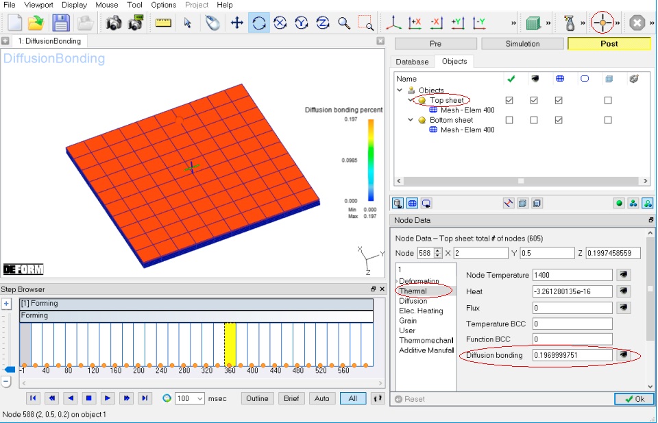
Contour of diffusion bonding percent at a selected step
The simulation result, i.e., the variation of diffusion bonding percent with time is summarized in Fig. DBL1.13. The analytical solutions at 5 selected times (1, 3, 4, 4.5, 5 hours) based on DFORM DB model are also imposed on Fig. DBL1.13. The FEM simulation results agree well with the analytical solutions. For example, in FEM simulation, the bonding percent is 0.12 at 1 hour and 0.197 at 3 hours, which are the same as the data in Table 2. After 3 hours, the pressure changes from 0.145 ksi to 0.4351 ksi. In order to calculate the bonding percent under the new pressure, we need to determine the equivalent bonding time under the new pressure in terms of the existing bonding percent. According to Table 2, at 1400F and under the pressure of 0.4351ksi, n=0.003966, m=0.56097, the equivalent bonding time for bonding percent 0.197 is 1055.69 seconds. For the total bonding time of 4 hours, the equivalent bonding time under the pressure of 0.4351 ksi is 1055.69+3600 seconds, i.e., 4655.69 seconds. According to equation EQ(1), the bonding percent is 0.003966*(4655.69^0.56097), i.e., 0.453. Similarly, for the total bonding time of 5 hours, the equivalent bonding time under the pressure of 0.4351 ksi is 8255.69 seconds; as a result, the bonding percent is 0.625. Fig. DBL1.13. also shows that a higher bonding rate can be reached due to increase of pressure.
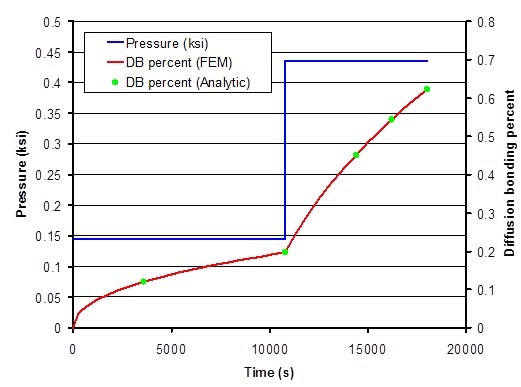
Variations of applied pressure and diffusion bonding percent with time