Material Suite Lab for deformation texture model

1.1. Abstract

1.2. Launch deformation texture model in material suite

1.3. Object selection and point selection

1.4. Setup for deformation texture model

1.5. Run material point simulator

1.6. Output

Abstract

Deformation texture model in material suite simulates the evolution of deformation texture at user selected interesting points after running a 2D or 3D nominal database. It can be applied to any single phase or dual-phase polycrystalline material. The crystal structure of each phase can be FCC, BCC, or HCP. DEFORM provides crystal plasticity (CP) executable (DEF_CP.EXE) or users can develop their own executables. For crystal plasticity executable provided by DEFORM, either Taylor or VPSC homogenization scheme can be employed. The texture can be represented either in Rodrigues space or Euler angles space. The basic input data include CP simulation control data, material definition, initial texture and microstructure. For each saved step in nominal database, the output data include macroscopic stress tensor of the polycrystalline aggregate, local stress components in each grain, and texture data, i.e., orientation distribution functions (ODFs) in Rodrigues space or Euler angles with weights. Texture analysis tools are provided, such as pole figures, inverse pole figures, and Kearns number of HCP crystal. For the nominal database with existing texture data, this module can be used to extract texture information and carry out texture analysis at user selected interesting points.

In this lab, the texture evolution of Ti-6Al-4V during forging is simulated.

Launch deformation texture model in material suite

On a Windows machine, go to the button, select DEFORM-v13.xxx (.xxx indicates version number E.g. v14.0.2 and select DEFORM GUI Main v1x.xx from the menu. The DEFORM GUI Main window will appear.

We require a nominal DB to perform texture analysis in material suite, for this lab we will use Double_Cone_Forging_Nominal.key from \MANUALS\PDF \DEFORM3D_Texture_Evolution_Lab folder to generate nominal DB. Open NG Pre using the link DEFORM GUI Main and define Problem ID as “ Double_cone_Forging “, select “3D “ Dimension radio button and “System International (SI) “ unit System radio button in New Problem window, then import Double_Cone_Forging_Nominal.key from \MANUALS\PDF \DEFORM3D_Texture_Evolution_Lab folder. Navigate to Generate DB page and click on to generate database. Close the NG Pre and run the simulation from GUI Main, make sure simulation stops normally without any issue. Now from GUI Main, without selecting **Double_cone_Forging.DB file click on **MaterialSuite under “Post Processor” to open Material Suite module.

After the main window for material suite pops up, click “Open…” icon ( ) in the top tool bar to import the example database (Double_cone_Forging.DB). The default task item “DEFORM” is added to the task tree. Expand “Microstructure” item and click “Texture Model” icon, the new task item “Texture evolution model” is added to the task tree.

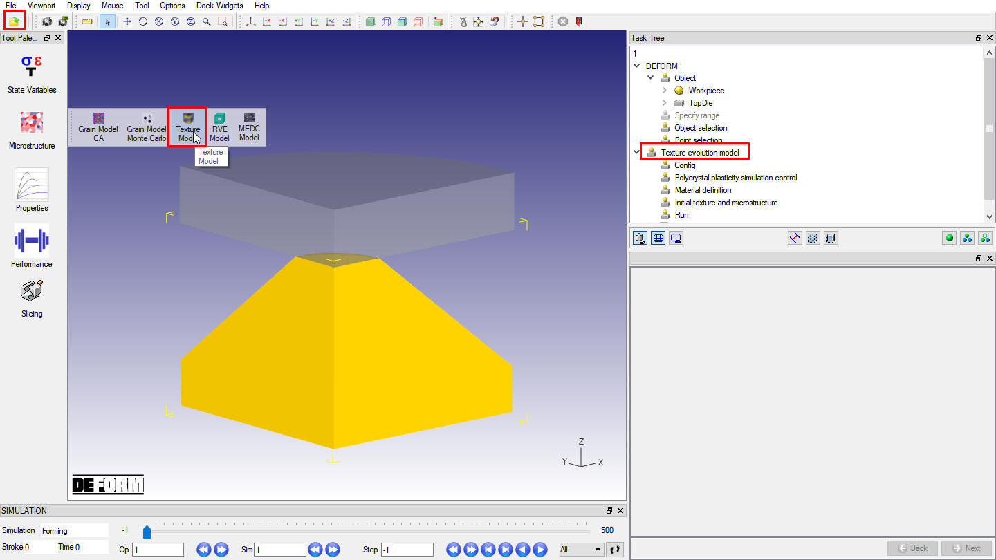
Launch deformation texture model in material suite.

Object selection and point selection

As shown in Fig. DTML1.2., in the “DEFORM” task tree, click “Object selection “ item and select “workpiece “. Click “Point selection “ item, define step number as “-1 “ and define two points on workpiece ( Fig. DTML1.3.). The coordinate of point 1 (P1) is (0.738, 0.147,0.967, 1) and the coordinate of Point 2 (P2) is (7.93, 0.071, 12.04, 1). Users can choose any step number convenient for them, such as the last step, to define the points.

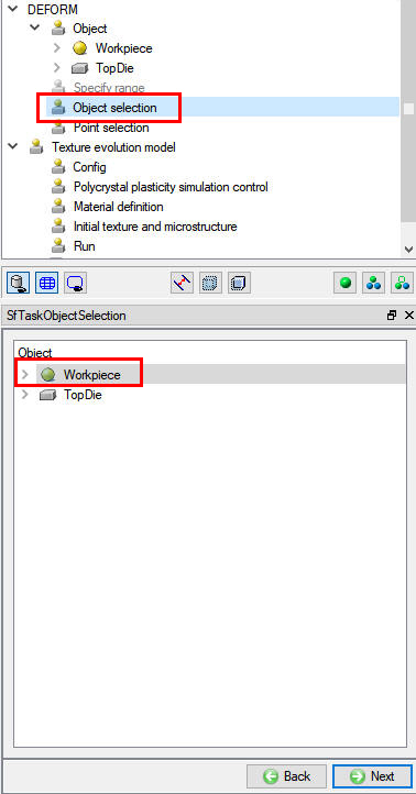
Object selection

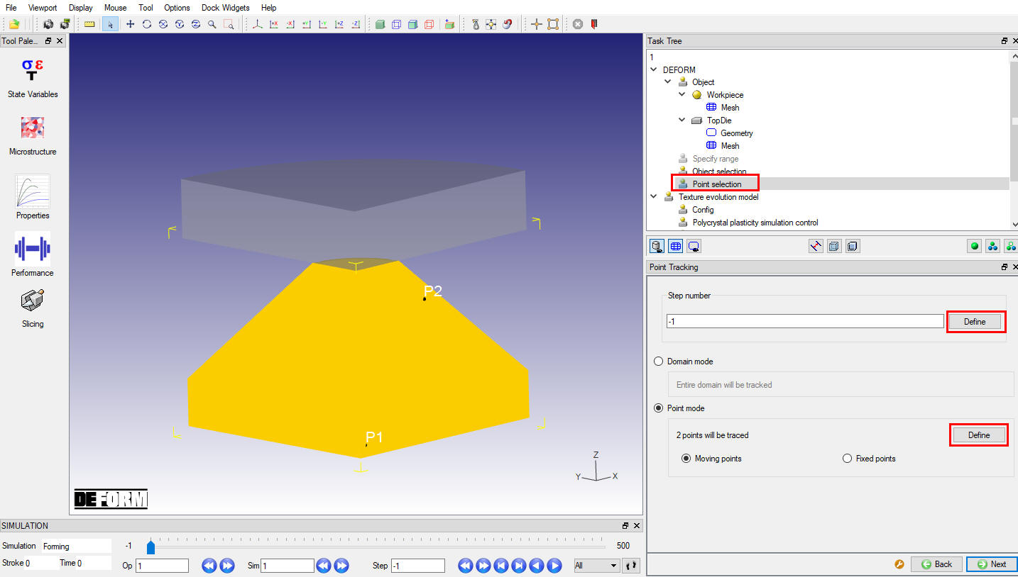
Point Selection

Setup for deformation texture model

All data for deformation texture model are prepared by the items listed in the “Texture evolution model “ task tree. Click “Config “ item, its data window appears as shown in Fig. DTML1.4. Specify the executable for CP simulation and the working directory by clicking the definition buttons (). The default executable for CP simulation implemented in DEFORM is “DEF_CP.EXE”, which is located at the installation directory of DEFORM software. Users can also develop their own executable for CP simulation and specify the file name here. The working directory must be the one where the nominal database is located.

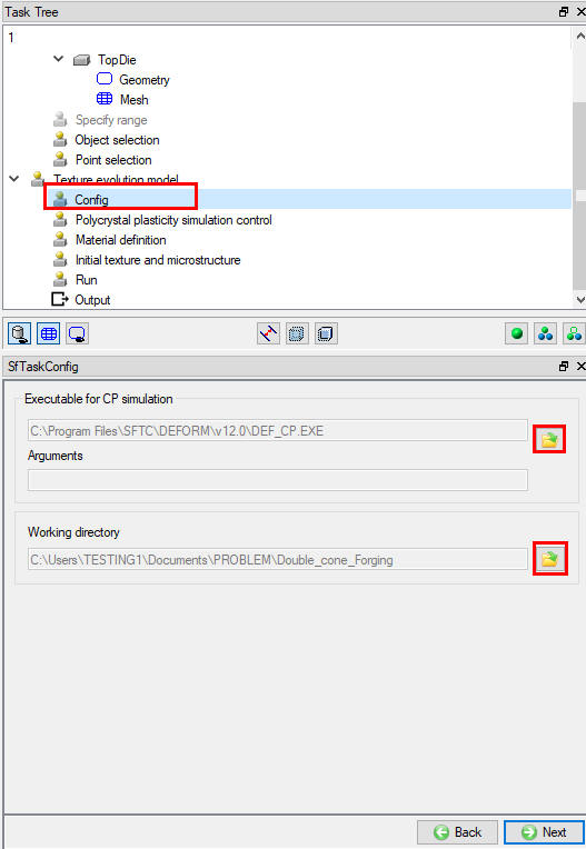
Configuration page

Click “Polycrystal plasticity simulation control “ item, its data window is shown in Fig. DTML1.5. The following data need to be specified: texture representation method (Euler angles or Rodrigues space), the step range to apply CP simulation, the source of texture data, the source of executable data, homogenization scheme (Taylor or VPSC), grain level linearization scheme (Secant, affine, intermediate, and tangent), convergence and iteration criteria. The default values are provided, but users can change these values. If the texture data (ODF) exist in the database, they can be detected automatically and GUI is setup accordingly, for example, “Existing ODF in database “ radio button is selected when texture data (ODF) exist in database. In this lab we will be using Texture representation method as Rodrigues space and source of texture data as New Definition since the nominal database does not have the ODF data. Specify the step range between -1 to 500. We will keep the Homogenization scheme to VPSC and Grain level linearization scheme to Affine and other fields are used with default values as shown in Fig. DTML1.6.

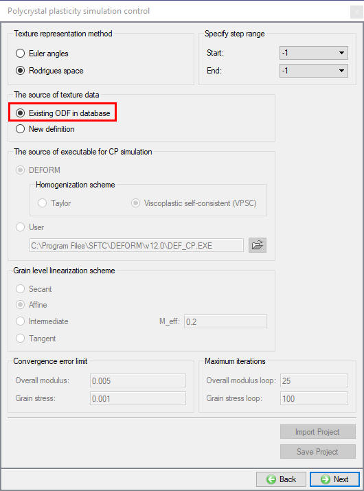
Polycrystal plasticity simulation control - Existing ODF in Database

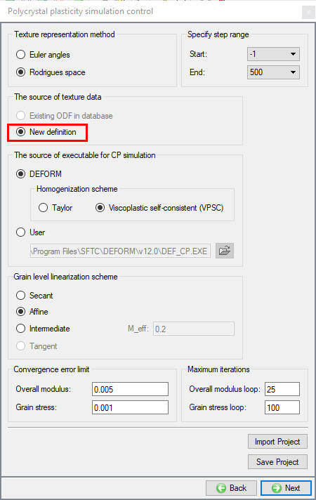
Polycrystal plasticity simulation control - New Definition

If the texture data exist in database, the material data are extracted automatically from database and displayed. The material properties can be viewed by clicking “Edit “ button. In this case, the material properties should not be changed. The only concerned property is the basic texture information (crystal type, texture type, and Rodrigues mesh type). If “New definition “ for texture source data is used in CP simulation control then it is necessary to redefine the material for the selected object . The new material for workpiece can be a single phase material or a mixture material. If it is a single phase material, we need to define its basic texture information and CP flow stress data (in plastic “ “ page), as shown in Fig. DTML1.8. and Fig. DTML1.9. If the new material for workpiece is a mixture material, we need to define the basic texture information and CP flow stress model data for each phase. Currently, only BCC (body-centered cubic), FCC (face-centered cubic), HCP (hexagonal close packed) crystal structures can be considered. Fig. DTML1.8. shows an example to define the CP flow stress model for an HCP crystal (like “Alpha” phase in Fig. DTML1.10.). For HCP crystal, we need to specify c/a ratio (like 1.588 for titanium alloys). The deformation mode is defined according to the family of slip plane and slip direction.

Since we are using “New definition” for texture source data in CP simulation control for this lab, it is necessary to redefine the material for the selected object (workpiece). Click “Material definition” item, an example keyword file with CP material parameters for Ti64 is located at the texture evolution lab folder (Ti64_LabTxr_CP.key). Import this keyword file using the “Import” button shown in Fig. DTML1.7. Imported material data can be viewed using Edit button. In this lab, we have two phases Alpha and Beta and for each phase we will use Rodrigues mesh type 2.

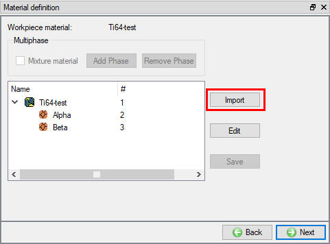
Material Definition

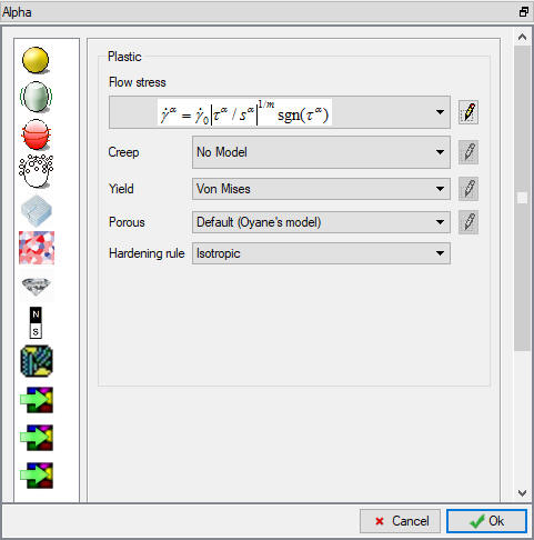
Material edit dialogue for Plastic property

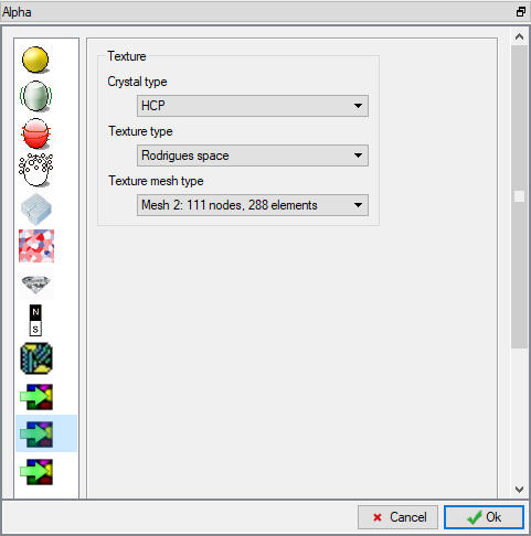
Material edit dialogue for basic texture information

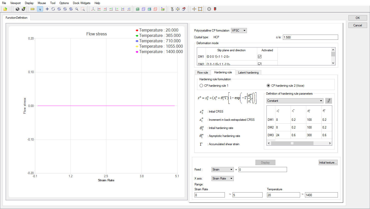
CP flow stress model for HCP crystal

In current DEFORM CP code, twinning deformation mode is not considered. HCP crystal has three deformation modes: basal slip (3 x {0001}<11-20>), prismatic slip (3 x {10-10}<11-20>), and pyramidal slip (6 x {10-11}<11-20> +12 x {10-11}<11-23> + 6 x {11-22}<11-23>). FCC crystal has one deformation mode: 12 x {111}<110>. BCC crystal has three deformation modes: 12 x {110}<111>, 12 x {112}<111>, 24x {123} <111>. All deformation modes are activated. The CP material parameters are defined for each deformation mode and latent hardening is defined among deformation modes. The CP material parameters can be constant or function of temperature. Two hardening rules are implemented in DEFORM. Hardening rule 1 is applied for Taylor scheme and hardening rule 2 is applied for VPSC scheme. The symbols in flow rule and hardening rule are briefly explained in GUI, and not repeated here. It is user’s responsibility to specify the appropriate CP material parameters, for example, obtaining from literature, determining by user’s own approach, or fitting by DEFORM flow stress module in material suite in terms of the experimentally measured flow stress data and initial microstructure (beyond the scope of this lab and not further discussed here).

Click “Initial texture and microstructure “ item to open its data window (Fig. DTML1.11.). If “Existing ODF in database “ is selected in the CP simulation control page, all data are automatically extracted and filled in this page. The data can be reviewed but not modified. Since “New definition” for texture source data is selected in the CP simulation control page, all data for each selected point should be defined here. The texture axes (RD-TD-ND) are defined in the global coordinate system for FEM simulation as shown in Fig. DTML1.11. Click on “Apply Axis “ button to apply the defined texture axis value for selected Point 1.

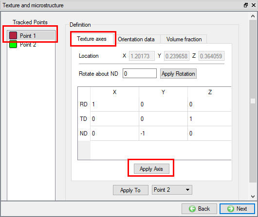
Initial texture and microstructure: texture axes

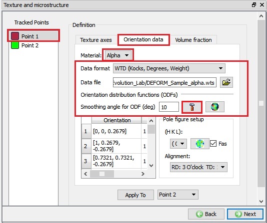
Click on Orientation Data tab, Fig. DTML1.12. shows the orientation data of alpha phase for a selected point (Point 1). If “Existing ODF in database “ in CP simulation control is selected, ODF values are extracted from database and displayed in the texture

table, which means that ODF values are represented in the RD-TD-ND system. If “New definition” is selected, we need to specify orientation data format, orientation data file, and smoothing angle (degree) for ODF (if the texture representation space

is Rodrigues space); then click the button (“”) to initialize texture data and display the result in the texture table. When the texture representation space is Rodrigues space, ODF values are calculated in the global coordinate system; when the texture representation space is Euler space, the Euler angles and weights in the RD-TD-ND system (as the received data) are displayed in the texture table. We can plot ODF contour and pole figures to examine whether the texture data are defined correctly.

Initial texture and microstructure: orientation data

In order to import the original texture data conveniently, five types of orientations or data formats are designed in DEFORM:

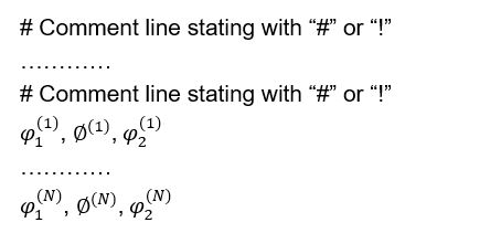
• Random orientation distribution, for which ODFs values are 1.0 at every independent node in Rodrigues space. For material with isotropic mechanical properties, this type of texture can be applied. If the texture representation space is Euler space, the corresponding Euler angles and weights are generated according to the basic texture information specified in “Material definition “ page.

• EBSD TSL/General (Bunge, radians)

The Euler angles are expressed in radians in Bunge’s notation. This is the default setting in DEFORM to calculate orientation matrix. The effective EBSD data (assuming the number of orientations is N) are rearranged in the following format:

• EBSD HKL (Bunge, degrees)

The Euler angles are expressed in degrees in Bunge’s notation. The effective EBSD data

(assuming the number of orientations is N) are rearranged in the following format:

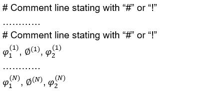
Before calculating the orientation matrix, the third Euler angles are added by 90 degrees in order to convert from HKL format to TSL format.

• WTD (Kocks, Degrees, Weights)

In “Weighted (WTD)” (Kocks, Degrees, Weights), the Euler angles are expressed in degrees in Kock’s notation. The effective weighted orientation data (assuming the number of orientations is N) are rearranged in the following format (Euler angles and weights):

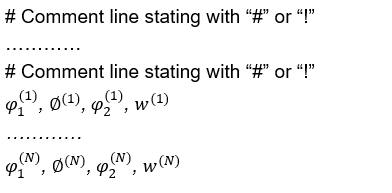
• WTD (Bunge, Radians, Weights)

In “Weighted (WTD)” (Bunge, Radians, Weights), the Euler angles are expressed in radians in Bunge’s notation. The data format is the same as in Type 4.

If the original experimentally measured texture data are not in these formats, user should convert the original data to one of the five designed formats, then import the converted data file. The ODF values in Rodrigues space depend on the smoothing angle, which is generally set as 5~10 degrees. Generally, the smoothing angle is set to 10 degrees for Rodrigues mesh type 2, 5 degrees for Rodrigues mesh type 3,and 2.5 degrees for Rodrigues mesh type 4.

In this lab, since we are using “New definition” we will define the smoothing angle of ODF to 10 degrees for both Alpha and Beta and click on . The initial texture data for alpha and beta are located in the texture evolution lab folder: DEFORM_Sample_alpha.wts , DEFORM_Sample_beta.wts. Data format type 4 (WTD: Kocks, Degrees, Weights) is adopted. Using option import Data file DEFORM_Sample_alpha.wt for Alpha material and DEFORM_Sample_beta.wts for Beta model .

Since we are using mixture material in this lab, the volume fractions for all phases need to be specified as shown in Fig. DTML1.13. in volume fractions tab.

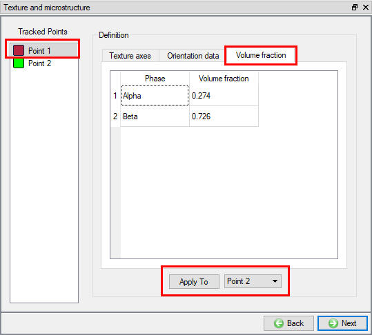
Initial texture and microstructure: volume fraction

After completing the definition of initial texture and microstructure for one point, we can click “Apply to “ button to copy the data to another point or all the remaining points if they have the same initial texture and microstructure. So, click on “Apply to “ to copy the data for Point 2 as shown in Fig. DTML1.13. After the setup for deformation texture model is finished, we can go back to the “Polycrystal plasticity simulation control “ page and click “Save project “ to save the project data. If there is a saved project setup, we can click “Import project “ button to load it.

Run material point simulator

Click “Run “ item in the task tree and click “Compute” button in the data window (see Fig. DTML1.14.). In the working directory, a folder named “TEXTURE” will be created, and under it, the folder for each selected point named “Point” ( denotes for point number) will be created to save the simulation results.

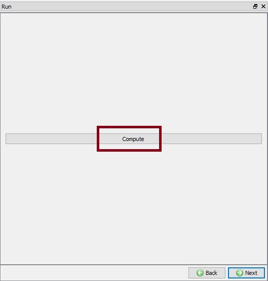
Run simulation

Generally, the following data files are created for each selected point. If user’s CP simulation executable is employed, the same input and output data file formats should be followed so that the texture analysis tools can import data correctly.

Input files for CP simulation executable:

STEP.txt: the saved step numbers in nominal database.

temp_mean.txt: The unit system and the history of temperature.

VELGRD.txt: The history of velocity gradient.

DEFGRD.txt: The history of deformation gradient.

SIMCTRL_CP.DAT: CP simulation control data.

MAT_CP.DAT: CP material parameters.

TxrInfo.txt: The basic texture information and initial volume fractions for all phases.

RDTDND.txt: The initial texture axes.

ODF_S-1.txt: The initial ODF values.

EulerAng_S-1.txt: The initial Euler angles and weights.

Output files from CP simulation executable:

ORM_S*.txt: The orientation matrix for individual grains at a saved step.

ODF_S*.txt: The ODF values at a saved step.

STRESS_LOCAL_S*.txt: The local stress components for individual grains at a saved step.

STRESS_MACRO.txt: The macroscopic stress components for polycrystalline aggregate at all saved steps.

For dual-phase titanium alloys, the following data files are generated:

DeformHis.Dat: deformation history data.

InitialTexture.Dat: The initial texture data for alpha phase and beta phase.

MATAX_S*.txt: Material axes at a saved step if they are defined in a database with existing ODF.

Output

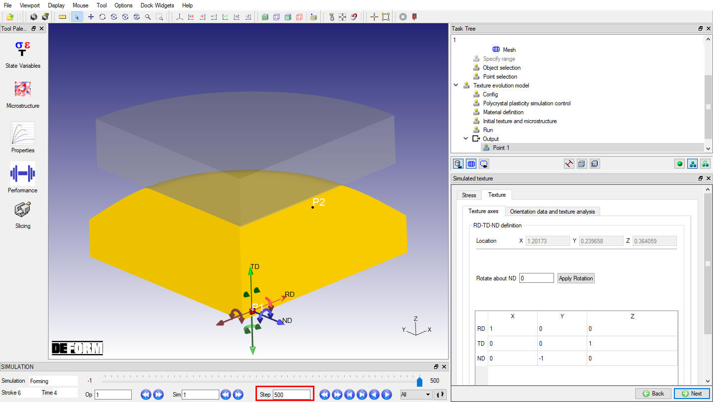
After simulation is finished, all the selected points are listed under the “Output” item in the task tree. Specify a step number in the step browser (should be within the range defined in the CP simulation control page) and select a point, the simulation results can be reviewed, as shown in Fig. DTML1.15. In order to carry out texture analysis, the texture axes need to be specified in the global coordinate system. Their values might be different from the initial texture axes defined in the “Initial texture and microstructure” page. In this example, the RD is aligned in global X direction, TD global Z direction, and ND global negative Y direction.

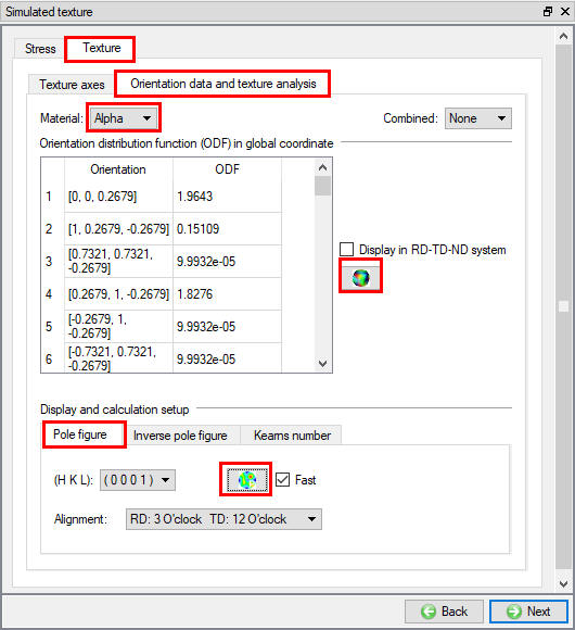
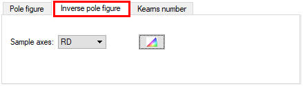
The orientation data for Point 1 at the last step is shown in Fig. DTML1.16. Using the provided texture analysis tools, we can plot ODF contour in Rodrigues space, pole figures, inverse pole figures, and calculate Kearns number of HCP phase. For BCC or FCC metals, 4 types of pole figures: (100), (110), (111), or all three pole figures can be plotted. For HCP metals, 4 types of pole figures: (0001), (11-20), (10-10), or all three pole figures can be plotted. The example results are shown in Fig. DTML1.16. - Fig. DTML1.21.

Output: Definition of texture axes for texture analysis

Output: orientation data and texture analysis tools to plot ODF contour - pole figures

Output: orientation data and texture analysis tools to plot ODF contour -inverse pole figures

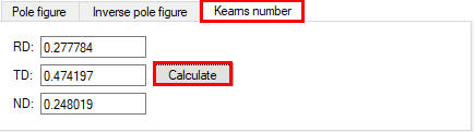
Output: orientation data and texture analysis tools to plot ODF contour - Kearns number

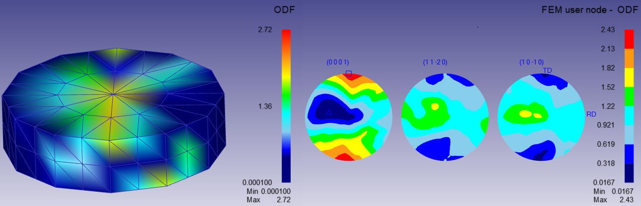
ODF contours (using values in table) and pole figures for Point 1 at the last step- alpha phase

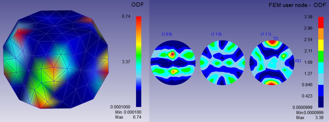
ODF contours (using values in table) and pole figures for Point 1 at the last step: beta phase

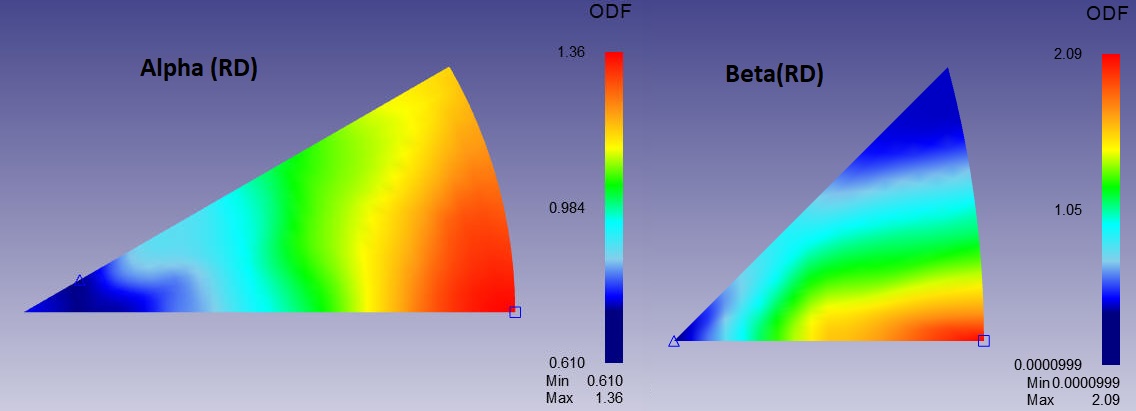
Inverse pole figures for RD for Point 1 at the last step for alpha phase