Add Cycles for 2D Operation

1.1. Introduction

1.2. Opening project file

1.3. Setting the MO Project

1.3.1. Operation 1 : Furnace operation

1.3.2. Operation 2 : Air transfer operation

1.3.3. Operation 3 : Rest on die

1.3.4. Operation 4 : Forming

1.4. Modifying the operation 4

1.5. Scheduled Positioning

1.6. Generate Database

1.7. Adding cycles

1.8. Cycles page

1.9. Post Processing

Introduction

The objective of this lab is to run a MO operation using cycles. If user needs to run the same deformation operation with multiple fresh parts using the same die set, we can use the ‘Cycle’ feature.

Opening project file

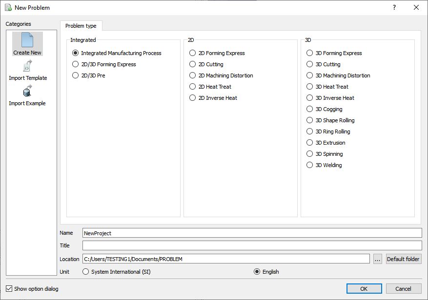
Create a new problem either by selecting File New Problem or by clicking the New Problem icon. The Problem Setup window will appear as shown in Fig. L1.1. Select “Integrated Manufacturing Process “ radio button and unit system as “English “ radio button in unit field. Define Problem Name as “ **Add_cycles_2D_lab1** “ and make sure the “Show option dialog ” check box is turned on (if we do not turn on the “Show option dialog” check box, then we will not get the New Project dialog). Then click on button to open a new problem using the Deform Integrated Manufacturing Process.

Problem defining window

MO wizard will open along with project naming window, defined problem name is updated as ‘Add_cycles_2D_lab1 ’ as the project name and selected unit system updated, click on to add project.

Setting the MO Project

Initially we will simulate the MO (multiple operation) problem with four operations (3 Heat transfer and 1 Forming operation) in batch mode then we will add cycles for the Forming operation. So add three 2D Heat transfer operations and one 2D Forming operation (see Fig. L1.2.).

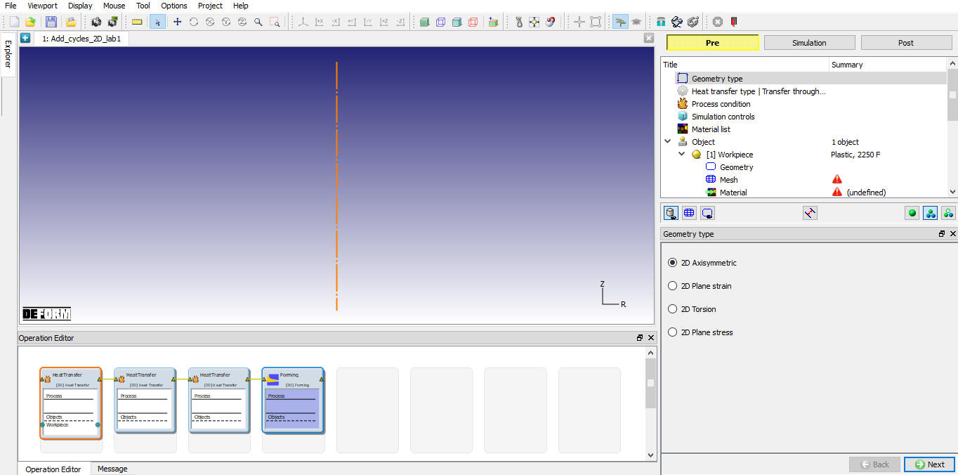
Adding Heat Transfer and Forming operations

Operation 1 : Furnace operation

Select Geometry type as 2D Axisymmetric.
Select heat transfer type as Heat in furnace.
In process condition page, define the Heating time as 3600 sec, Environment Temperature as 2000°F and Convection coefficient as 7.7e-6 Btu/sec/in^2/F.
Turn on Heat transfer check box only in the Simulation controls page.
In Material window, load the material AISI -8620 from DEFORM Material library, from Steel category using (Load material data from library) option.
Add only one object in the Objects page.
In workpiece page define the workpiece temperature as 68°F.
In Workpiece Geometry page, click on (Load Geometry from Library) button and import ‘Disk_wkp.igs ’ from 2D\LABS Location. Check and correct the geometry using option.
Generate the mesh using 2000 elements.
To assign material for workpiece select the material ‘AISI-8620 ’ from material window.
In step controls page, Set the number of simulation steps as 100 at 36sec each and saving every 10 steps
Generate the DB and click to go to next operation.

Operation 2 : Air transfer operation

Select heat transfer type as Transfer through Air.
In process condition page, define the Transfer time as 15 sec, Environment Temperature as 68°F and Convection coefficient as 7.7e-6 Btu/sec/in^2/F.
Since workpiece is a Read from DB object we don’t have to define any other object properties.
In Step Controls window define number of steps as 15 at 1 sec increment and saving at every 5 steps.
Visit the DB generation page and click to go to next operation.

Operation3 : Rest on die

Select heat transfer type as Rest on die.
In process condition page, define the Transfer time as 4sec, Environment Temperature as 68°F and Convection coefficient as 7.7e-6 Btu/sec/in^2/F.
In Top die Geometry page, click on ( Load Geometry from Library) button and import ‘Disk_top.igs ‘ from 2D\LABS Location. Check and correct the geometry using option.
Generate the mesh using 600 elements.
In Top die material page, load the material AISI-H13 from DEFORM Material library.
In Bottom die Geometry page, click on ( Load Geometry from Library) button and import ‘Disk_btm.igs ‘ from 2D\LABS Location. Check and correct the geometry using option.
Generate the mesh using 600 elements.
In Bottom die material page, select the material AISI-H13 from material window.
Position the Top die using Offset positioning (x=0, y=4) towards Y direction.
In scheduled positioning page, define the bottom die Position as interference positioning with respect to workpiece in Y direction.
Add one relation in contact page as Bottom die as Master and Workpiece as slave, Click on button, select Free resting in the pull down menu for the Heat transfer coefficient under Thermal tab.
In Step Controls window define number of steps as 10 at 0.4 sec increment and saving at every 2 steps.
Visit the DB generation page and click to go to next operation.

Operation 4 : Forming

In objects page, add three Objects.
In workpiece page, select the Read from DB radio button.
Similarly, select Read from DB radio button for other two objects also.
In Top die Movement page, assign a constant die movement of 1 in/sec in the negative ‘Y’ direction.
In scheduled positioning page, define the Top die Position as interference positioning with respect to workpiece in negative Y direction.
In contact page for all default relations, define the Hot forming (lubricated) from the list. A friction value of 0.3 will automatically be selected.
In step controls window, define the number of steps as 100, at 0.0725” per step of die movement, step increment to save as 10 for the primary die (which is object number 2 in this operation).
Visit the DB generation page, save the project and select the tab.
Start the simulation by clicking the action label, use the default Continue Run option to select “Continue from the last step ” option and then select the Simulation mode as Interactive and click on button.
After the completion of the simulation switch to Post to post processing.
After post processing switch to preprocessor by clicking tab.

Modifying the operation 4

In the tab, select the operation 4 (Forming operation) and click until Workpiece page.

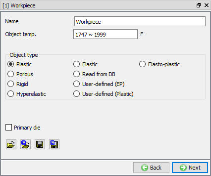
Workpiece

In the workpiece page change the object type to plastic from Read from DB (see Fig. L1.3.). When we change the object type to plastic we will see the workpiece object of the 4th operation first step. Click until Scheduled Positioning page.

Workpiece page

Scheduled Positioning

In the scheduled positioning page, we must make sure that top die is scheduled to position on the top of the workpiece. Click until DB generation page.

Generate Database

Click on action label to check the problem. Generate a database by clicking action label.

When we click on the, we will get a popup of Lost steps, it will ask that all steps available under 4th operation will be lost if we generate the database. Click for the popup. (see Fig. L1.4.)

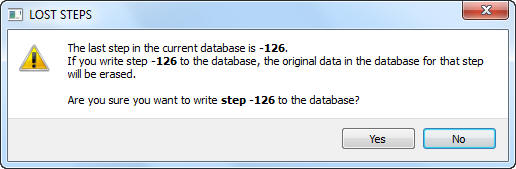
Lost steps popup

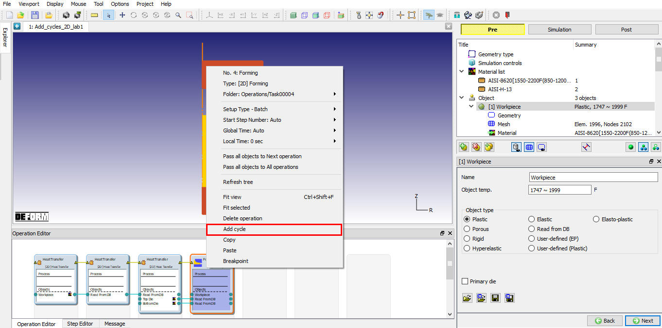
Adding cycles

After generating DB select the operation editor, right click on the 4th operation and select the Add cycles. (see Fig. L1.5.)

Adding Cycles

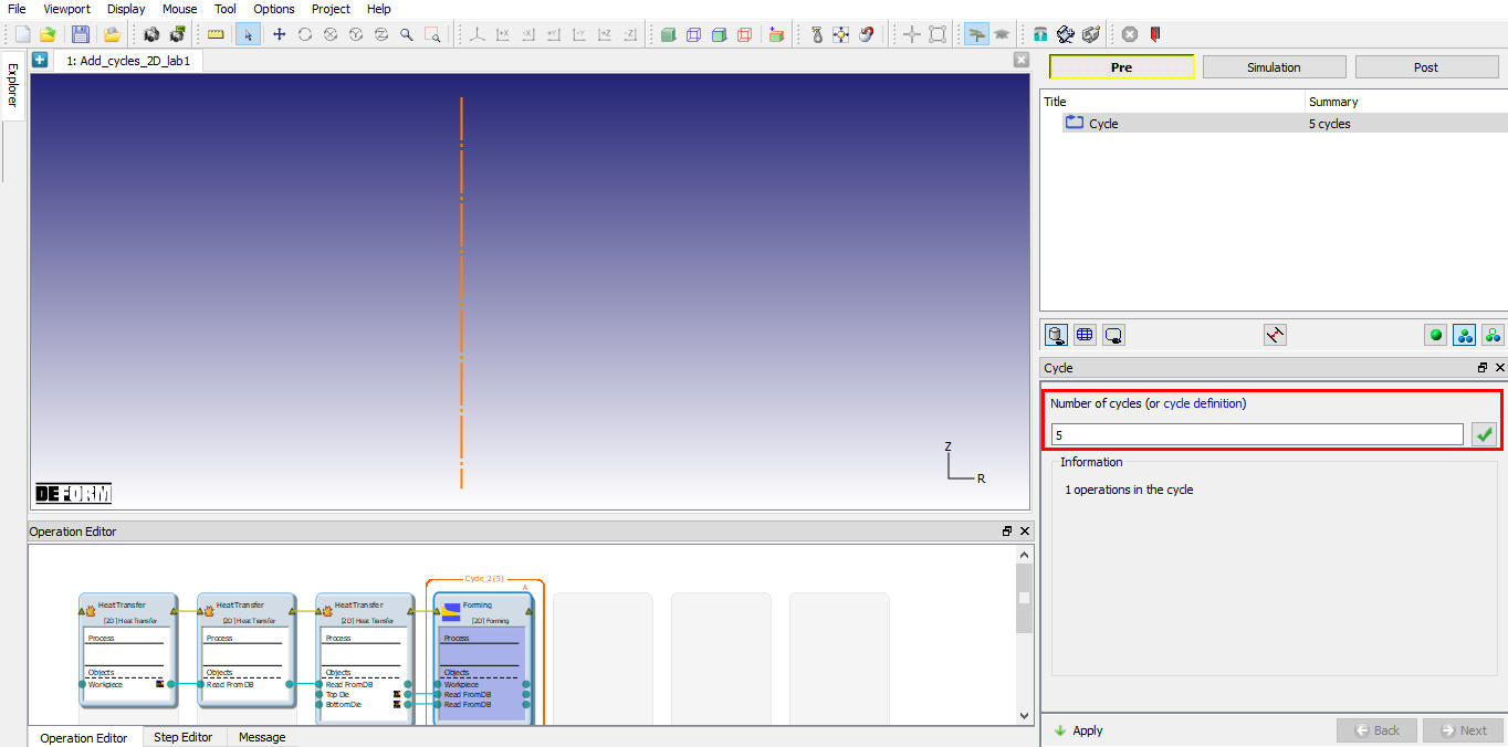
Cycles page

After adding Cycles click on apply to accept the default number of cycles as 5 and save the wizard (see Fig. L1.6.). Switch to the Simulation mode by selecting the button above the object tree. Click on the action label to open the Run Options dialog as shown in Fig. L1.7. Use the default Continue Run option to select “Continue from the last step ” option and then select the Simulation mode as Interactive and click on button to run the simulation.

Add cycles window

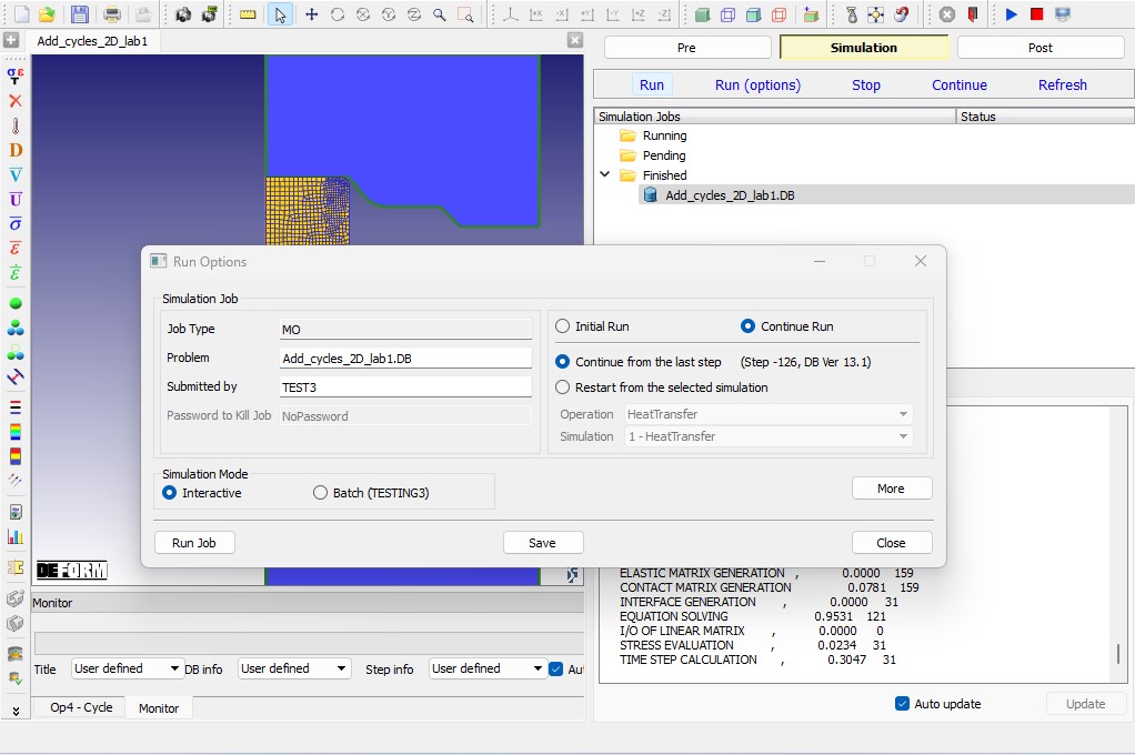
Simulation mode window

Post Processing

In step Browser, we can see the steps of Cycles operation (see Fig. L1.8.). Play the steps to see all cycle operations.

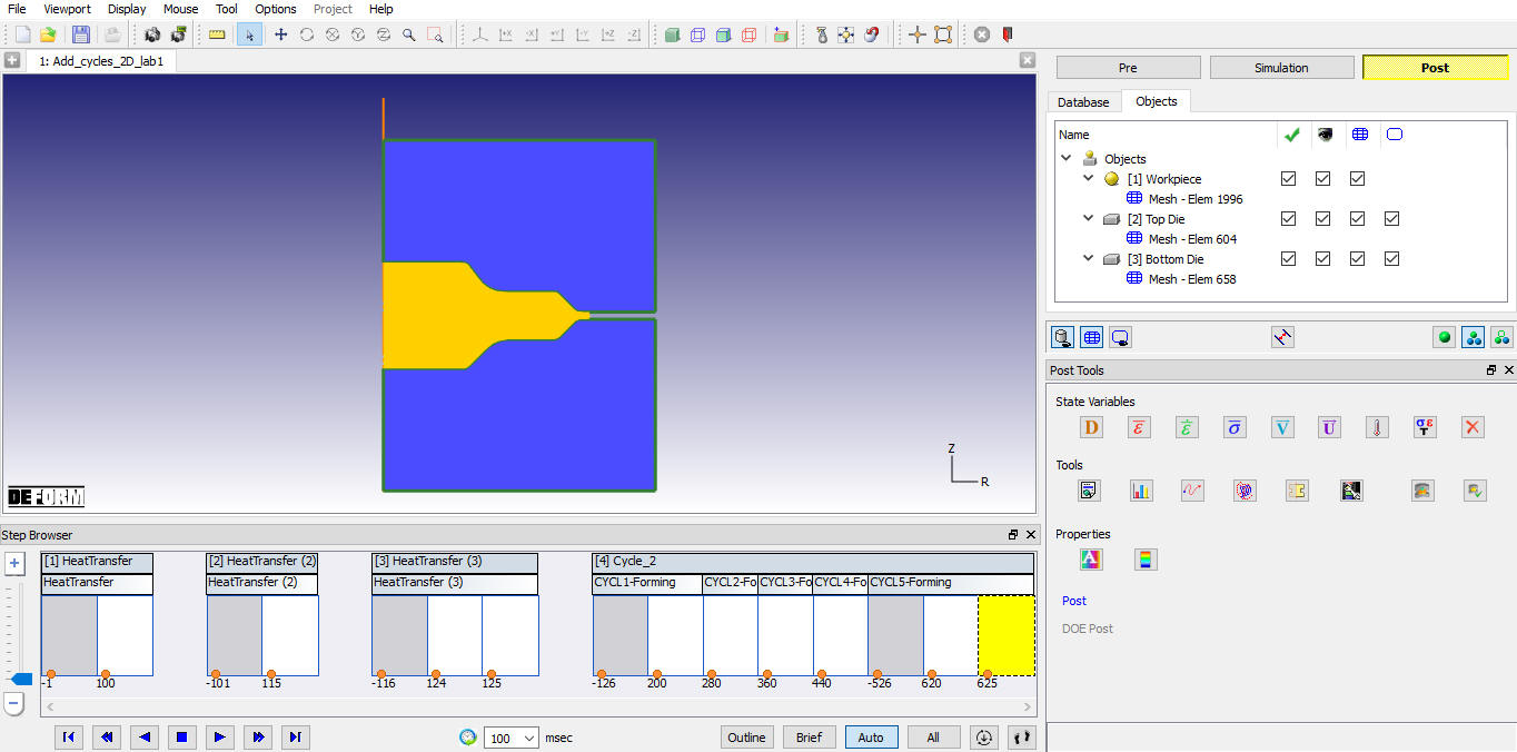
Post window

State Variable:

Select Strain-Effective from post tools to look at the amount of deformation the workpiece has undergone. Click the icon to bring up the State Variable window, select Strain-Effective state variable, select Solid shading by clicking on Solid display button and select as the Scaling option. This option will use the Local Min and Max effective strain as the extremes on the color bar. Scaling, Shading and other contour plot setting can also be changed from RMB options on Color bar. Play through the steps of the simulation to observe the accumulation of strain (see Fig. L1.9.). Temperature plot shows the workpiece temperature along with dies temperature, since we made the dies as read from DB objects in forming operation, same dies used for all cycle operation and we can see the temperature change of dies for cycle operations (see Fig. L1.11.).

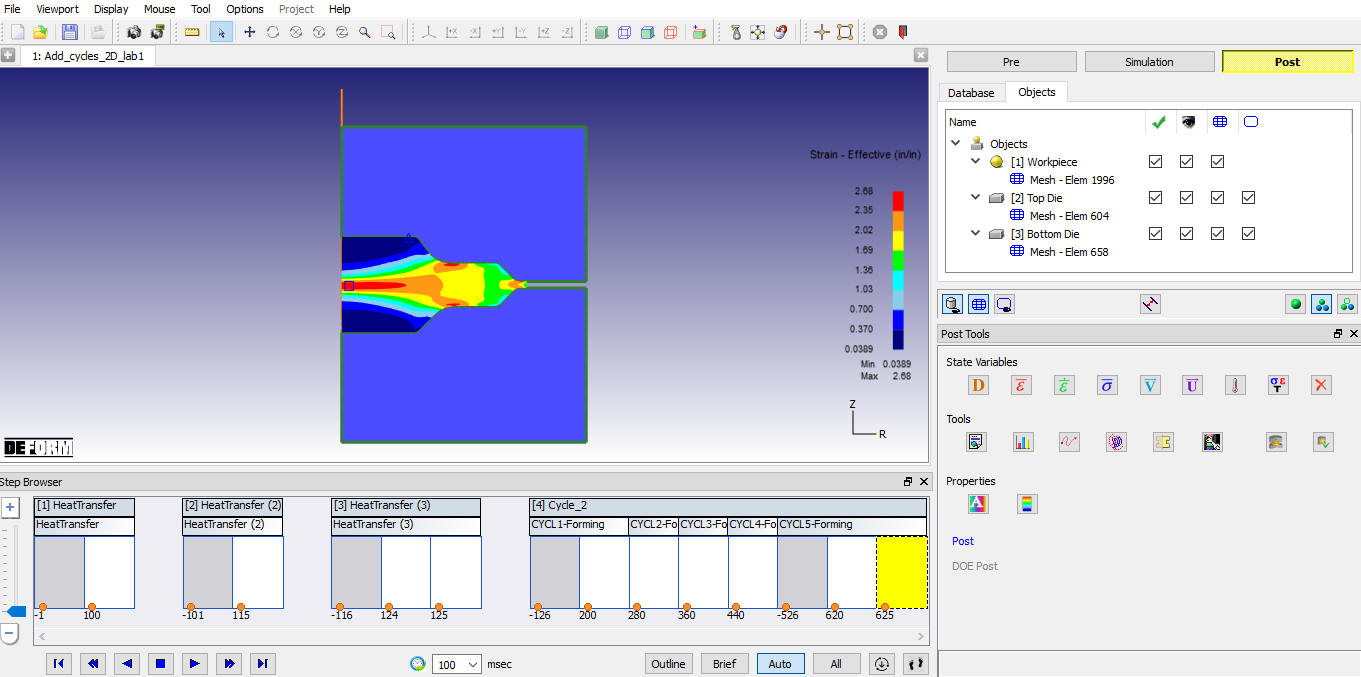
Strain effective plot

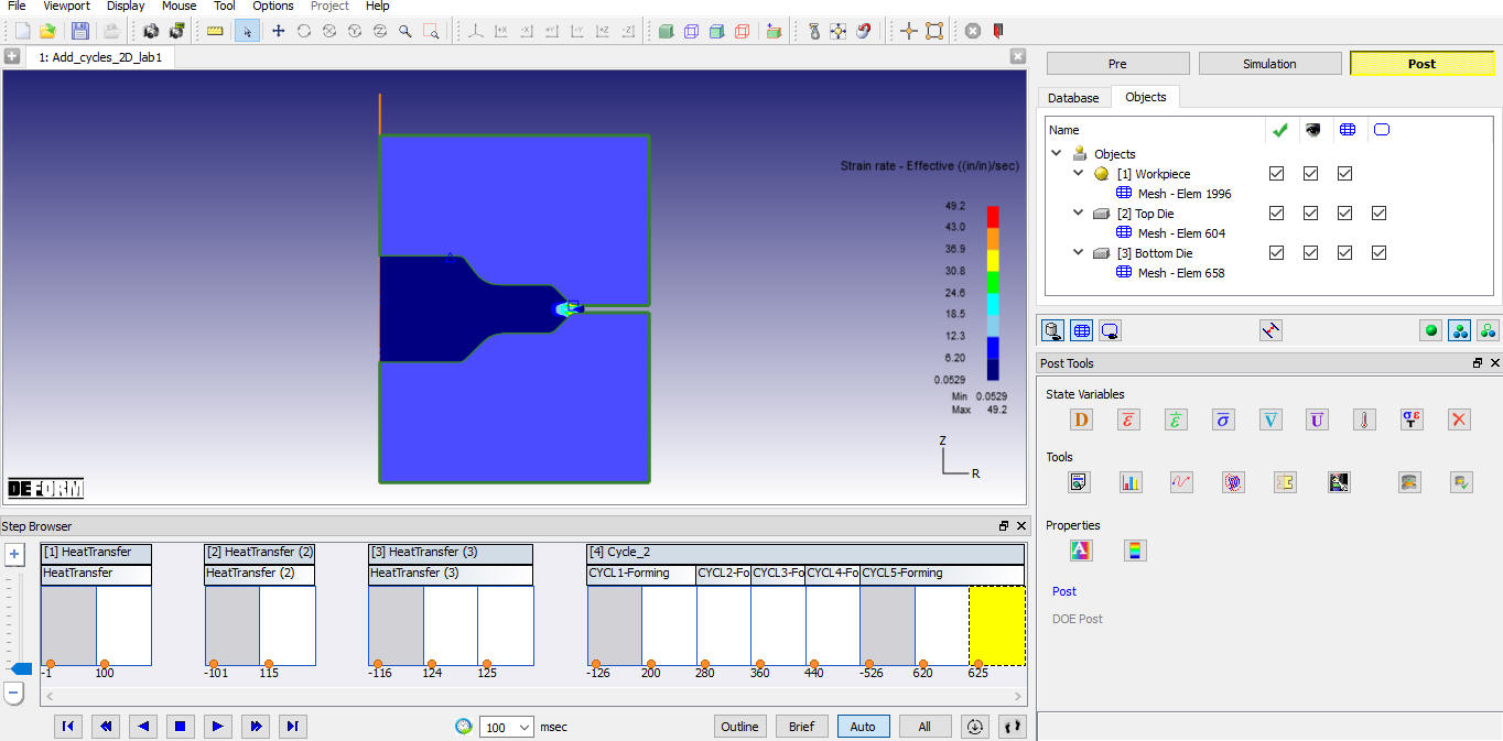
Stress Effective plot

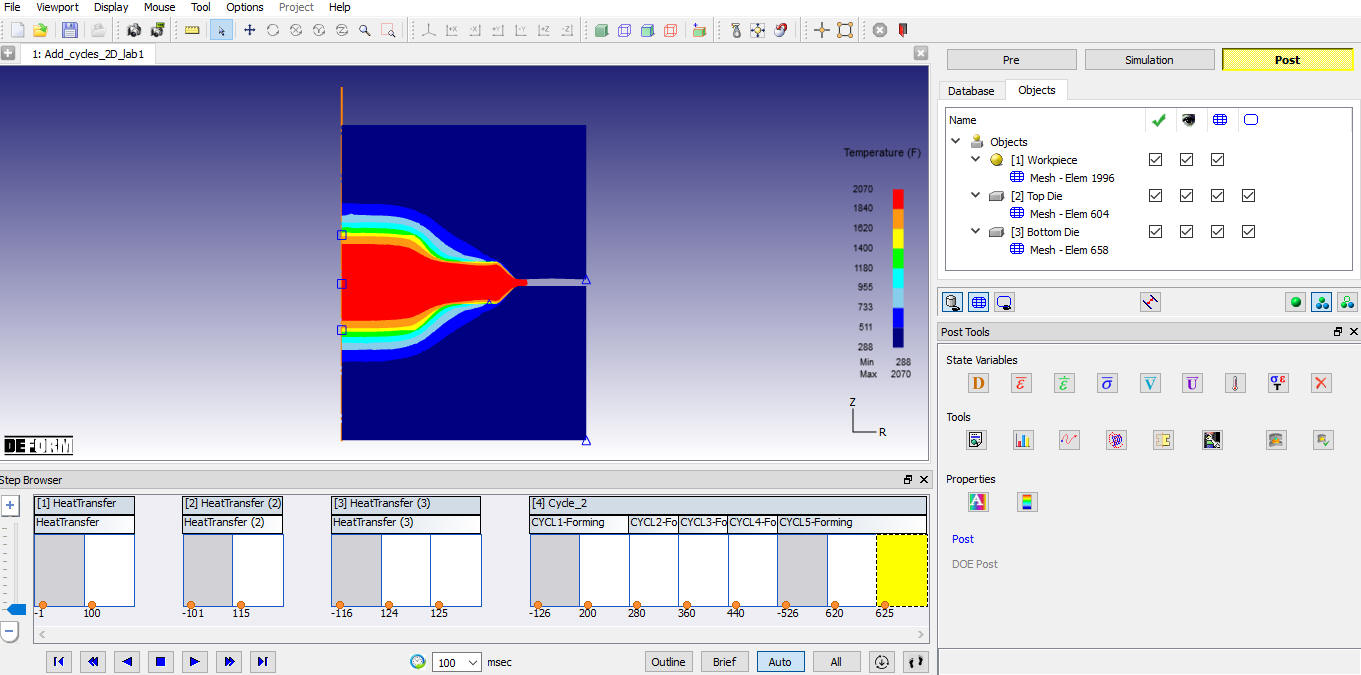
Temperature plot