Swaging Lab1
In this lab for quarter symmetry 3d model Infeed swaging operation setup is demonstrated using ICFG example.
1.1. Creating New Problem
1.2. How to add 3D Swaging operation
1.3. Define Swaging Process Settings
1.4. Define pass table data
1.5. Load material
1.6. Define Workpiece Object
1.7. Define Top die Object
1.8. Defining Inter-object relations
1.9 Preview the Swaging pass
1.10. Define Simulation controls
1.11. Check and Generate Database
1.12. Submit to Simulate
1.13. Post process the Results
1.14. Setting up the Swaging Explicit setup
Creating New Problem
Create a new problem either by selecting File ![]() New Problem or by clicking the New Problem
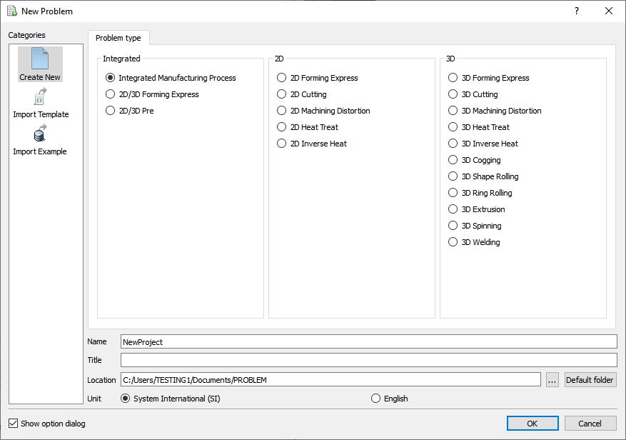
New Problem or by clicking the New Problem ![]() icon. The Problem Setup window will appear as shown in Fig. 3DSWL1.1. Select “Integrated Manufacturing Process “ radio button and unit system as “SI “ radio button in unit field. Define Problem Name as “**Swaging_ICFG_Ex** “ and make sure the “Show option dialog” check box is turned on (if we do not turn on the “Show option dialog ” check box, then we will not get the New Project dialog in MO UI). Then click on
icon. The Problem Setup window will appear as shown in Fig. 3DSWL1.1. Select “Integrated Manufacturing Process “ radio button and unit system as “SI “ radio button in unit field. Define Problem Name as “**Swaging_ICFG_Ex** “ and make sure the “Show option dialog” check box is turned on (if we do not turn on the “Show option dialog ” check box, then we will not get the New Project dialog in MO UI). Then click on ![]() button to open a new Problem using the Deform Integrated Manufacturing Process.
button to open a new Problem using the Deform Integrated Manufacturing Process.
Opening New Problem
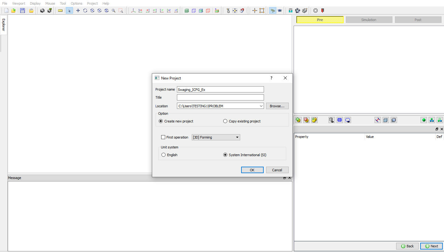
Multiple operation wizard will open with the New Project dialog as shown in Fig. 3DSWL1.2., at this point user will be prompted to specify a project name (system will create a separate folder with this project name) and title for this session. In Problem Name popup define Problem Name as “Swaging_ICFG_Ex “ as the project name as shown in Fig. 3DSWL1.2.
Add new Project Name and Unit System
How to add 3D Swaging operation
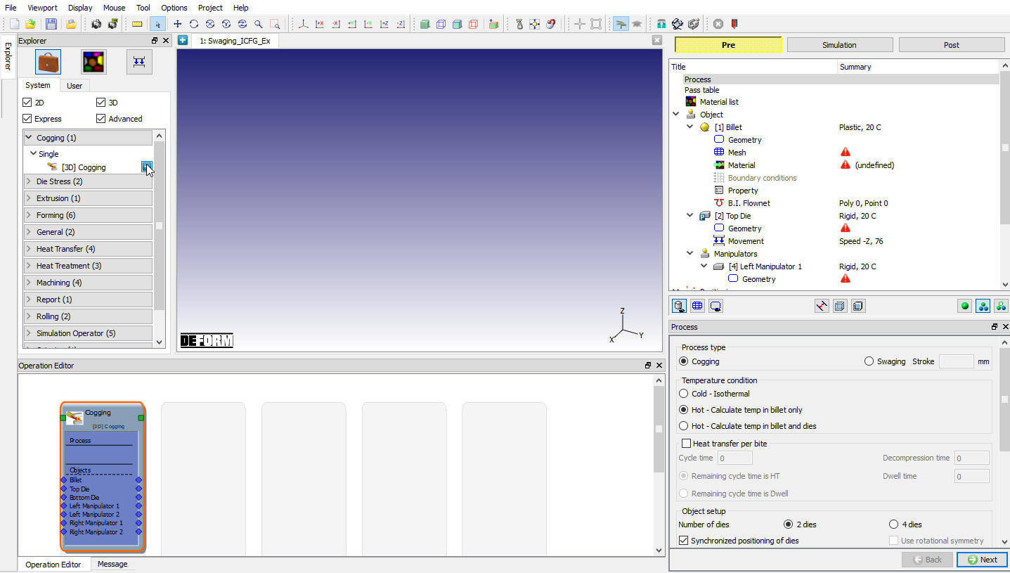
Add swaging operation from MO explorer by clicking on ![]() button next to Cogging operation or user can also add by drag and drop into the Operation Editor as shown in Fig. 3DSWL1.3.
button next to Cogging operation or user can also add by drag and drop into the Operation Editor as shown in Fig. 3DSWL1.3.
Add Swaging operation from operation explorer
Define Swaging Process Settings
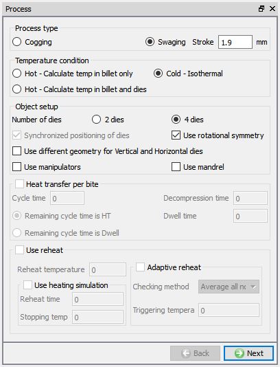
Select the Swaging process type radio button and enter the stroke value as1.9 mm as shown in Fig. 3DSWL1.4. User must enter the swaging stroke value so it stops the simulation after each bite if it crosses the stroke of primary die in movement direction.
Swaging Process window
As this is cold forging operation select temperature calculation as Cold-Isothermal. Select 4 dies and uncheckUseManipulators checkbox they are normally used in cogging operation to hold the workpiece.
For symmetric setup select Use Rotational Symmetry checkbox this gives the respective geometry primitives and generates the necessary boundary conditions by default. Click ![]() to define the swaging pass data.
to define the swaging pass data.
Define pass table data
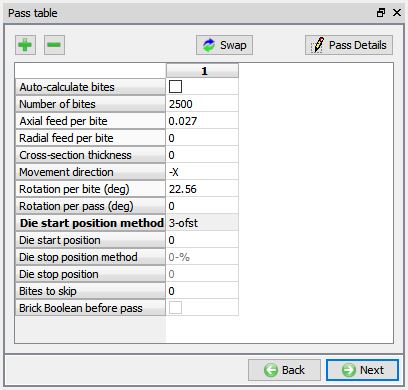
Swaging entire pass information like Number of bites, Axial die feed per bite, Radial die feed per bite, Die Movement direction, Workpiece rotation per bite, workpiece rotation per pass and die positioning can be entered in pass table. New pass can be added by using the icon similarly added pass can be deleted using icon. Pass information is copied from previous pass whenever a new pass is added and necessary information can be edited based on the process requirement.
Enter number of bites as 2500 , Die Axial feed per bite 0.027 mm, workpiece rotation per bite to 22.56 , leave the Die movement direction as –X and selectDie start positioningmethod as “3-ofst “ as shown in Fig. 3DSWL1.5.
Click ![]() to load the material for workpiece.
to load the material for workpiece.
Pass table information
Load material
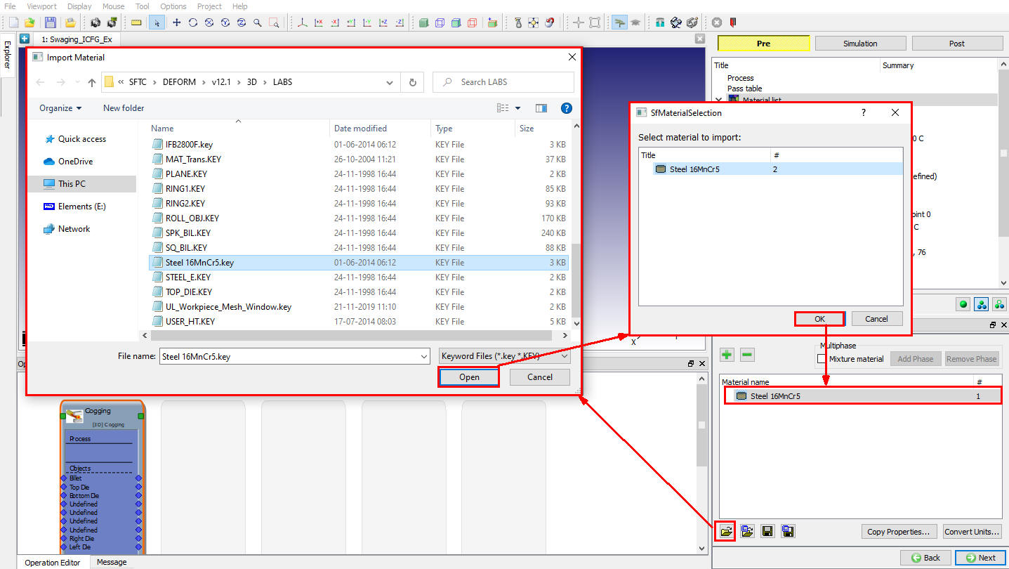
Load the material “Steel16MnCr5 ” from DEFORM installation path \3d\LABS\ folder “Steel 16MnCr5.key “ file using ![]() (load material from file) option, system popups a dialog with material list and list is the materials available in the keyword file as there is only one material in key file click
(load material from file) option, system popups a dialog with material list and list is the materials available in the keyword file as there is only one material in key file click ![]() as shown in Fig. 3DSWL1.6.
as shown in Fig. 3DSWL1.6.
Load material from file
Click ![]() until Object window leaving the defaults as axial subdivision is intended for cogging where huge deformation takes place and click
until Object window leaving the defaults as axial subdivision is intended for cogging where huge deformation takes place and click ![]() to go for Workpiece object window.
to go for Workpiece object window.
Define Workpiece object
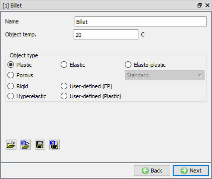
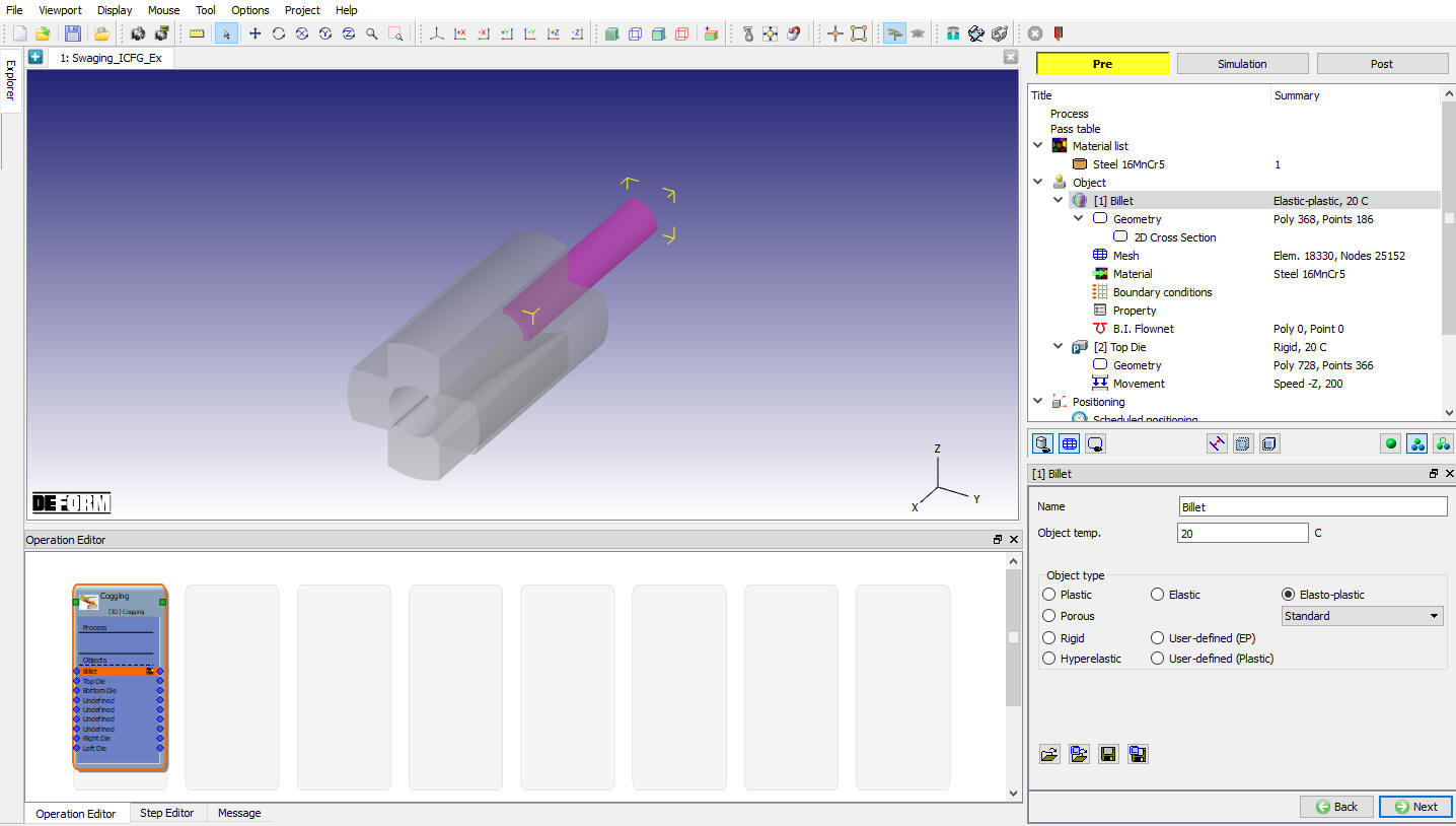
Leave the object name as Billet and default object type Plastic as it is. Assign the temperature to 20 °C as shown in Fig. 3DSWL1.7. Click ![]() to define the Geometry for billet.
to define the Geometry for billet.
Billet object window
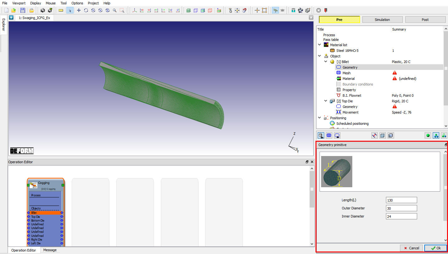
Define Billet Geometry
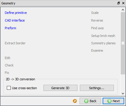
Click on ![]() geometry option to define the geometry using primitives as shown in Fig. 3DSWL1.8.
geometry option to define the geometry using primitives as shown in Fig. 3DSWL1.8.
Geometry window
Enter the Length130 mm, Innerdiameter24 mm and Outerdiameter30 mm to create the symmetric geometry as shown in Fig. 3DSWL1.9. Click ![]() to close the Geometry Primitive.
to close the Geometry Primitive.
Billet 3D Geometry
Click ![]() for 2D Cross-section window and observe the 2D geometry extracted from the 3D geometry used for brick mesh generation as shown in Fig. 3DSWL1.10.
for 2D Cross-section window and observe the 2D geometry extracted from the 3D geometry used for brick mesh generation as shown in Fig. 3DSWL1.10.
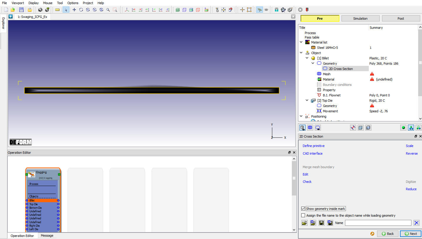
Billet 2D extracted geometry
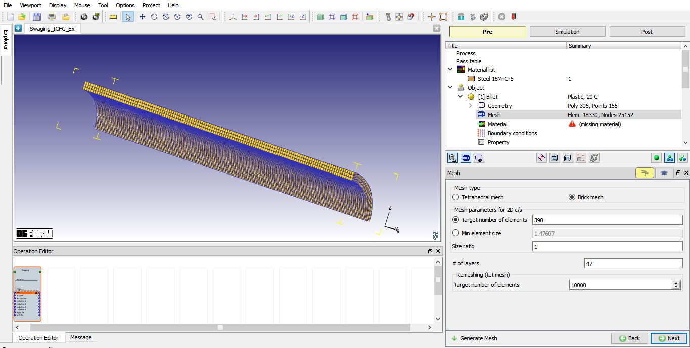
Define Billet Mesh
Select brick mesh radio button and enter number of elements to 390 , Size ratio 1 and # of layers to 47 and generate the mesh clicking on ![]() button and click
button and click ![]() in “Default Boundary conditions” popup.
in “Default Boundary conditions” popup.
For 2D cross section geometry as observed in Fig. 3DSWL1.10. system generates 390 mesh elements and revolve about 90 deg in 47 layers as shown in Fig. 3DSWL1.11. Click ![]() to Material page.
to Material page.
Billet mesh window
Assign Material for Billet
Select the loaded material “Steel16MnCr5 ” from material list to assign it to workpiece as shown in Fig. 3DSWL1.12.
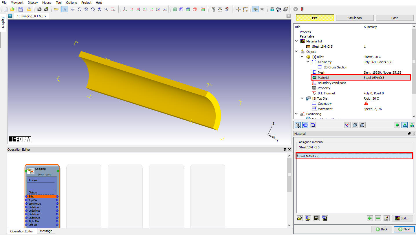
Assign billet material
Define Boundary Conditions
Observe the system assigned default rotational symmetry BCC and Fixed velocity at the free end of the billet BCC as shown in Fig. 3DSWL1.13. and Fig. 3DSWL1.14. Click ![]() until Top die page to define Top die.
until Top die page to define Top die.
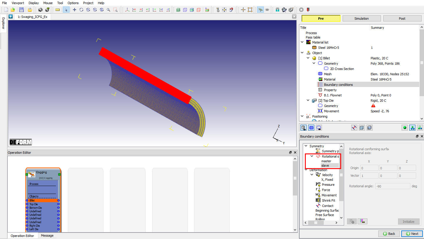
Rotational Symmetry BCC
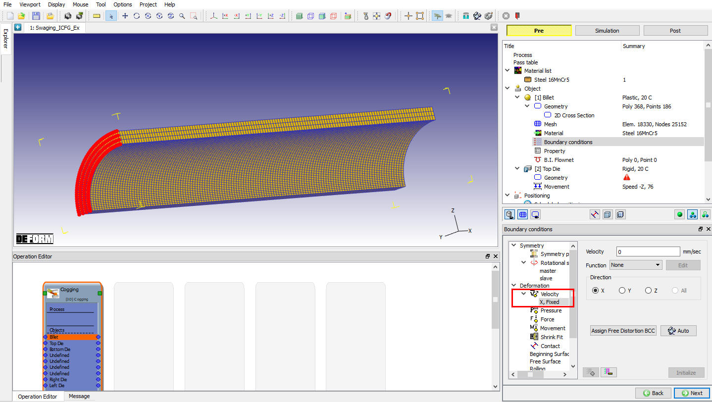
Velocity BCC
Define Top die Object
Leave the object name as Top die and default object type Rigid as it is and assign the temperature to 20 °C as shown in Fig. 3DSWL1.15. Click on ![]() .
.
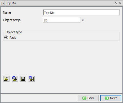
Top die object page
Define Die geometry
Import the Die geometry Swaging_ICFG_Die_SI.stl from installation path \3d\LABS\ folder as shown in Fig. 3DSWL1.16.
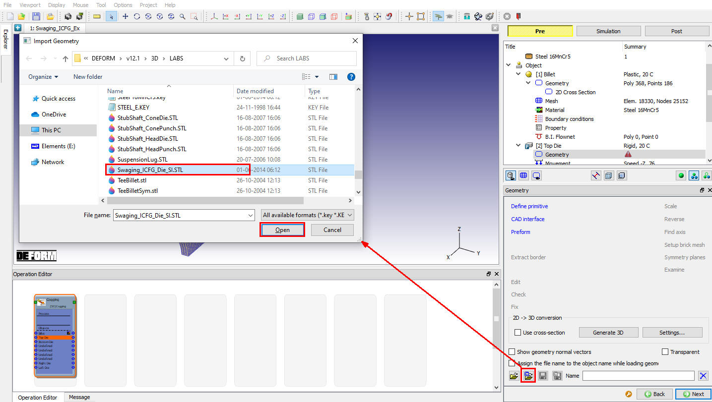
Importing Die geometry
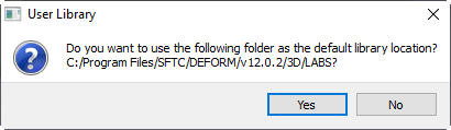
For User library popup asking to use the current geometry file browsed location as default library location. By default 3d LABS path will geometry library path, so click ![]() .(See Fig. 3DSWL1.17.)
.(See Fig. 3DSWL1.17.)
User Library path update
Observe the imported geometry internal profile showing the Inlet feed angle, Calibration Length and Outlet Run out angle as shown in Fig. 3DSWL1.18.
Note: If the Die needs positioning, then user should select the Die positioning method as “3-offset” in Pass Table page. This allows user to position the Die.
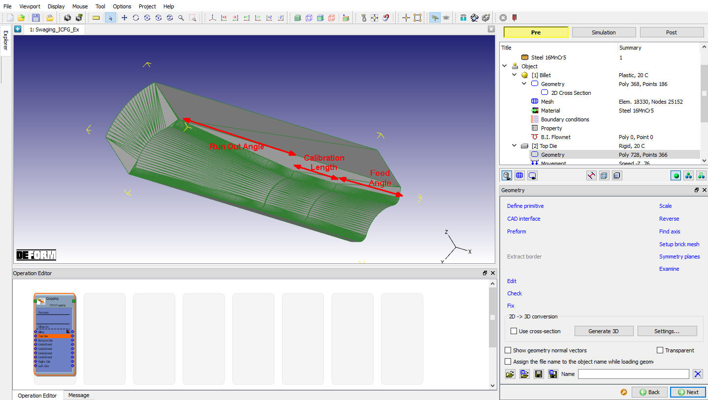
Imported Die geometry
Define Die movement
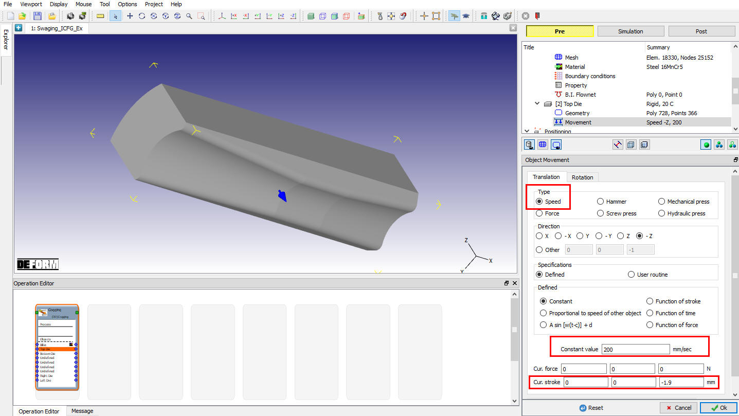
Select Advanced radio button type and click on ![]() button, define the die movement as constant Speed as 200 mm/sec and set theCurrent Stroke as -1.9 , since the die geometry is imported in its closed position as shown in Fig. 3DSWL1.19. Click on
button, define the die movement as constant Speed as 200 mm/sec and set theCurrent Stroke as -1.9 , since the die geometry is imported in its closed position as shown in Fig. 3DSWL1.19. Click on ![]() to close Advanced movement page.
to close Advanced movement page.
Die movement window
Defining Inter-object relations
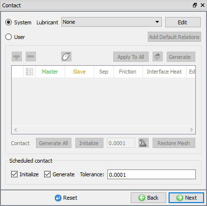
Click ![]() until Contact page as the swaging operation automatically position dies around the workpiece at equal angles manual position is not needed. Select System contact definition type and check scheduled contact Initialize and Generate check boxes and enter small contact tolerance value 0.0001 as shown in Fig. 3DSWL1.20. System will generate the contact automatically during database generation. Click
until Contact page as the swaging operation automatically position dies around the workpiece at equal angles manual position is not needed. Select System contact definition type and check scheduled contact Initialize and Generate check boxes and enter small contact tolerance value 0.0001 as shown in Fig. 3DSWL1.20. System will generate the contact automatically during database generation. Click ![]() until Simulation preview page.
until Simulation preview page.
System type Inter-object settings
Preview the Swaging pass
Observe the Die and workpiece movement and positioning preview by playing with step manipulation options. Click ![]() to Simulation controls controls.
to Simulation controls controls.
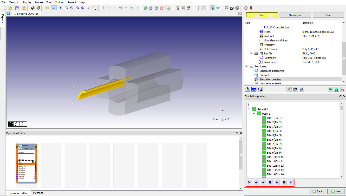
Swaging preview window
Define Simulation controls
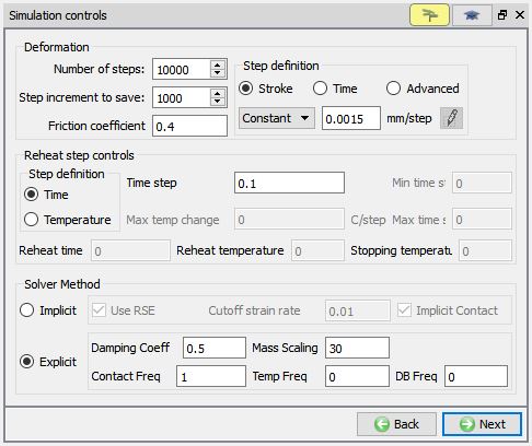
Enter the number of steps to 10000, step increment to save to 1000 and 0.0015 mm stroke/step as shown in Fig. 3DSWL1.22. In addition to this friction coefficient value 0.4 is defined will be used in contact friction calculation. Implicit solver is used to solve this setup. Leave the implicit solver default settings. To know more about RSE and Implicit contact refer and respectively.
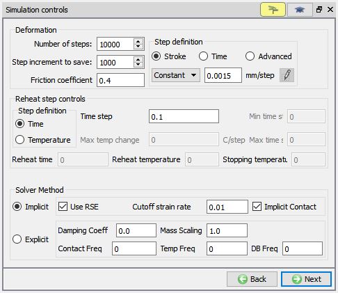
Simulation control window
Check and Generate Database
Click on ![]() and observe the message tab for DB checking messages, if there is any input errors will be indicated by red color and also display the warning messages. Error message block the user to generate DB. Confirm the DB checking is OK and click on
and observe the message tab for DB checking messages, if there is any input errors will be indicated by red color and also display the warning messages. Error message block the user to generate DB. Confirm the DB checking is OK and click on ![]() . (See Fig. 3DSWL1.23.) After generating Database switch to Simulation mode by clicking on
. (See Fig. 3DSWL1.23.) After generating Database switch to Simulation mode by clicking on ![]() button.
button.
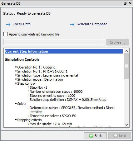
Generate Database window
Submit to Simulate
Click on the ![]() action label to open the Run Options dialog as shown in Fig. 3DSWL1.24. Use the default Continue Run option to select “Continue from the last step ” option and then select the Simulation mode as Interactive and click on
action label to open the Run Options dialog as shown in Fig. 3DSWL1.24. Use the default Continue Run option to select “Continue from the last step ” option and then select the Simulation mode as Interactive and click on ![]() button to run the simulation.
button to run the simulation.
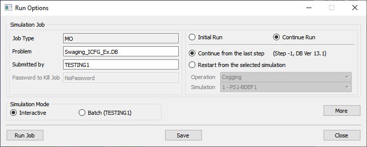
Submit to simulate
User can use more processors and run in 64 bit by using the ![]() . As the simulation starts simulated saved steps will update in simulation graphics window and also Message and LOG files display the status of the current simulation as shown in Fig. 3DSWL1.25.
. As the simulation starts simulated saved steps will update in simulation graphics window and also Message and LOG files display the status of the current simulation as shown in Fig. 3DSWL1.25.
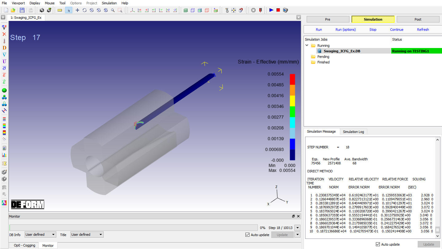
Monitor using simulation graphics
Simulation completion or stop will be indicated in the message file. After completion of the simulation click on ![]() tab to post process the DB.
tab to post process the DB.
Post process the Results
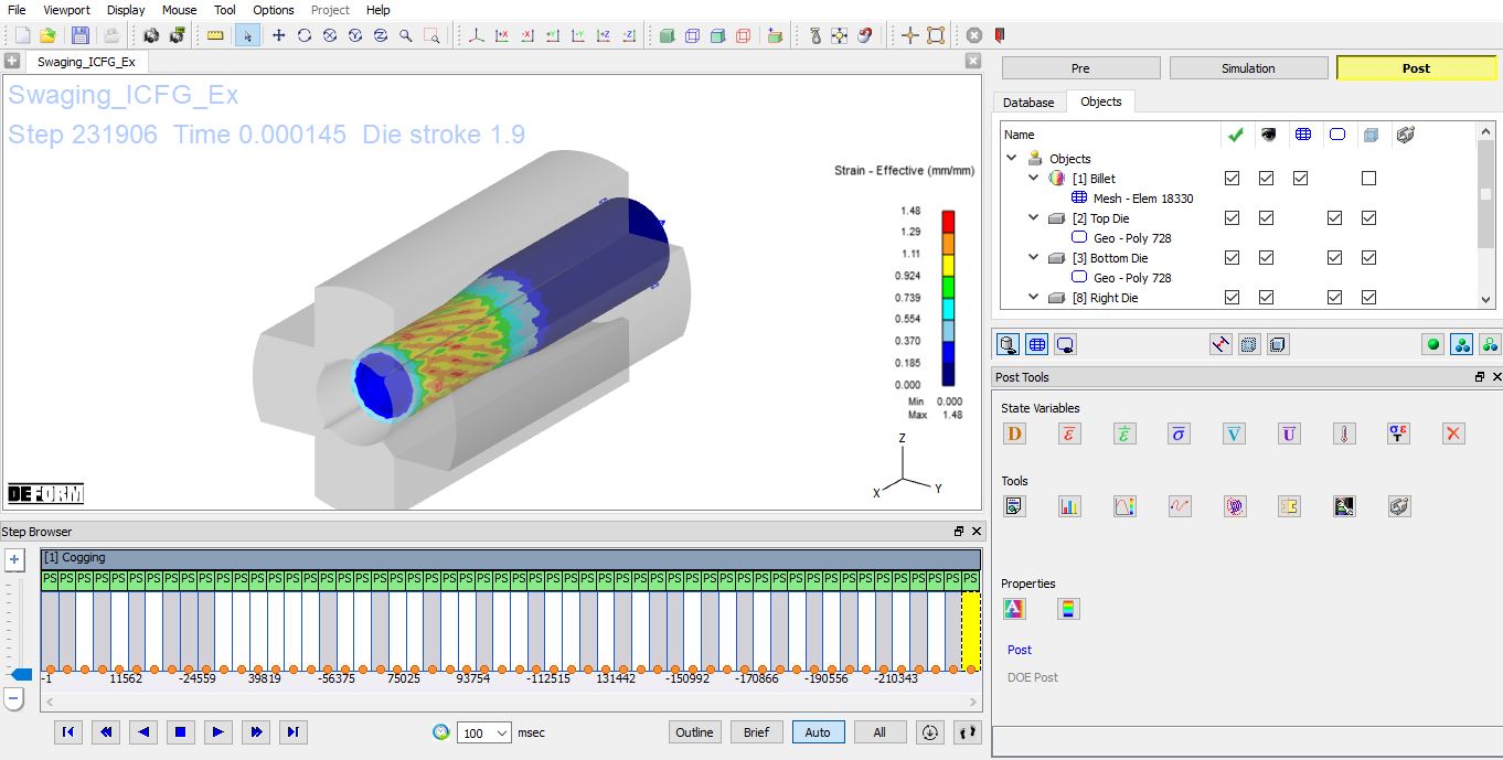
Play through the Steps and see the Strain distribution by plotting the effective strain State variable. (See Fig. 3DSWL1.26.)
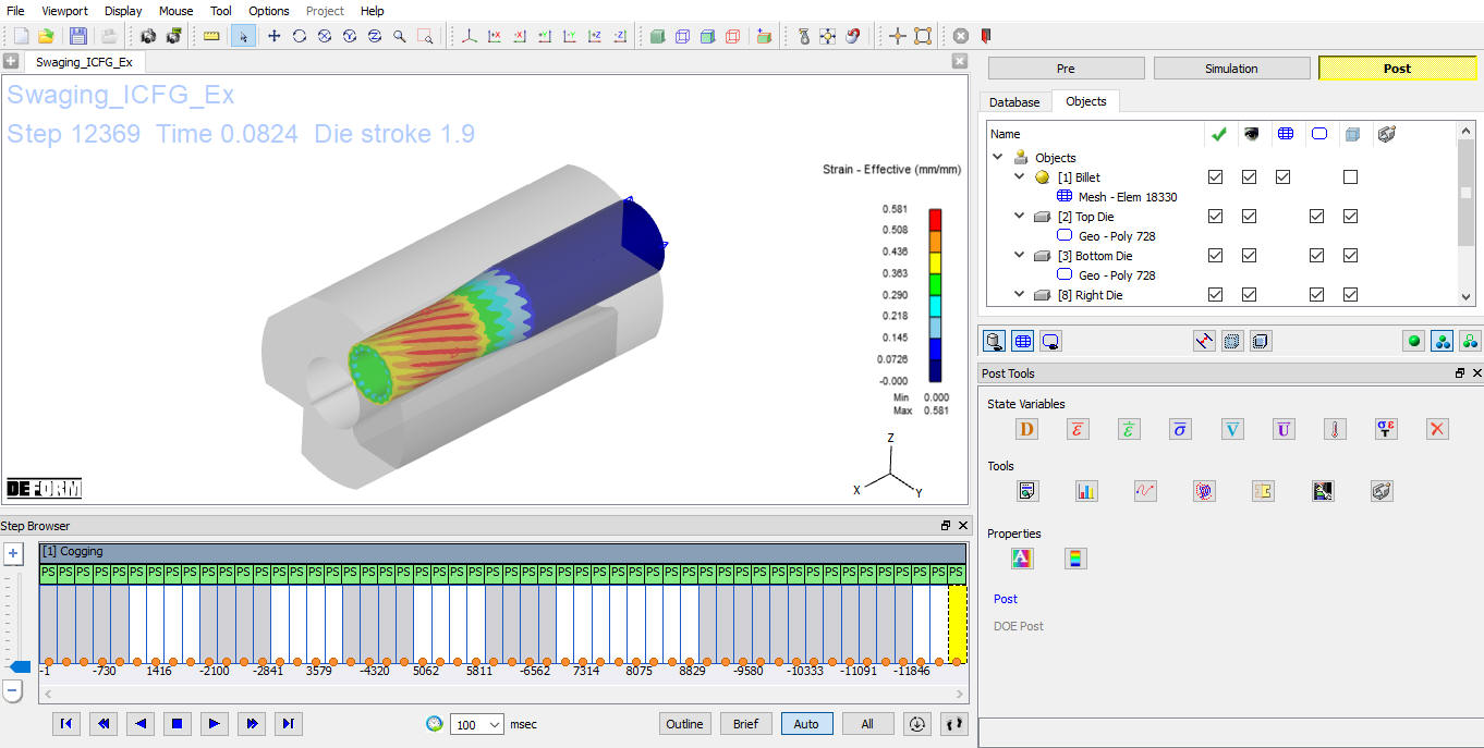
Strain Distribution
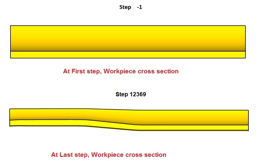
Workpiece cross section thickness
Setting up the Swaging Explicit setup
In Explicit solver make workpiece asElasto plastic object by visiting back to Billet object window as shown in Fig. 3DSWL1.28.
Billet Object selected as Elasto plastic object
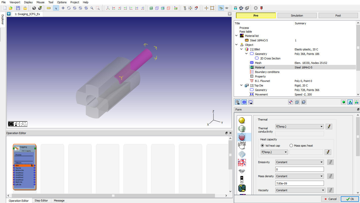
After making the billet as Elasto plastic go to workpiece material page, click on ![]() define the Massdensity as 7.85e-09 under Thermal tab as shown in Fig. 3DSWL1.29. Click on
define the Massdensity as 7.85e-09 under Thermal tab as shown in Fig. 3DSWL1.29. Click on ![]() to close the material edit page.
to close the material edit page.
Defining Mass density data
Go to S**im ulation controls** window and select Explicitsolver method radio button as shown in Fig. 3DSWL1.30. Enter the Dampingcoefficient as 0.5 , Mass scaling as 30 and Contact Frequency as 1.
Simulation controls for Explicit solver method
Click ![]() to go the Database generation window and check and generate the Database to submit to simulate in Next steps. Similar to the section 1.12. and 1.13. submit the generated DB to simulate and post process using MO post respectively.
to go the Database generation window and check and generate the Database to submit to simulate in Next steps. Similar to the section 1.12. and 1.13. submit the generated DB to simulate and post process using MO post respectively.
Plot Strain Effective at last step for the Simulated Database (See Fig. 3DSWL1.30. and Fig. 3DSWL1.31.)
Strain effective plot
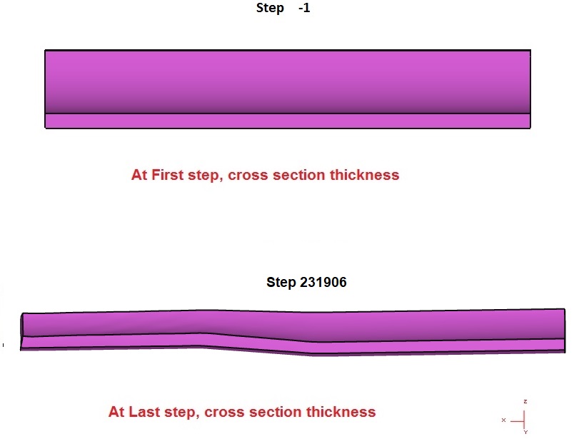
Workpiece cross section
Related Topics: