Appendix I : Elementary Concepts in Metal forming and Finite Element Analysis

AI.1. Definition of stress, strain and strain rate

AI.2. Introduction to FEM theory

AI.3. Modeling Material Behavior in FEM

Definition of stress, strain and strain rate

Stress is the measure of force applied per unit area. This variable is of importance in forming, in that material deform (change shape) different amounts depending on how much stress they are under. There are several definitions of stress.

Engineering Stress - The engineering stress is defined as force per unit area measured on the original undeformed shape.

True Stress - The true stress is defined as the ratio of the applied force to the instantaneous cross-sectional area. These two definitions are shown in Fig. AI.1 as a comparison. In general, the true stress is more interesting for an engineer in analyzing a forming process. True stress will indicate plastic yielding and other issues with better accuracy than engineering stress.

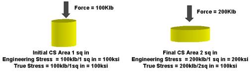
Demonstration of concept of stress

Strain is a measure of the total accumulated deformation a region of material has undergone.

Mathematically, the two definitions of this are seen as follows:

Engineering Strain = (Change in Length) / (Original Length)

True Strain = Sum of incremental strains = ln ( (final length) / (initial length))

In Fig. AI.2., the calculated strains for both an upset and a tensile test are shown. Note that the Engineering strain gives rather round numbers for doubling or halving the length of a test specimen. The advantage of true strain is that it is a more accurate measure of the actual length change in the material and is used to determine stress in DEFORM.

Strain rate is a measure of the instantaneous rate of deformation a region of material is experiencing. This quantity measures a rate of change of the strain at a point of a material per unit time.

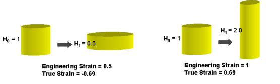
Demonstration of concept of strain

In Fig. AI.3., the engineering stress and strain are shown as closed form expressions for a compression test. Note that both of these quantities fail to account for the increase in area of the test specimen due to barrelling.

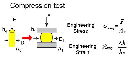
Engineering stress and strain for a compression test

In Fig. AI.4., the true stress and strain are shown as closed form expressions for a tension test. Note that both of these expressions account for the change in the cross-sectional area of the specimen during the test (assuming incompressible material). This gives a better measure of the actual state of stress and strain the material is under.

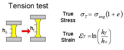
Stress and strain defined for tension test

All materials have a characteristic stress-strain curve that determines how the material behaves structurally. For most isotropic metals, this behavior is of the general shape as seen in Fig. AI.5. Note that the top and bottom curves are the engineering stress-strain curves for a material and the middle curve is the true stress-strain curves for a given material. The true stress-strain curve is the same for either tension or compression, but they are not the same in terms of engineering stress-strain.

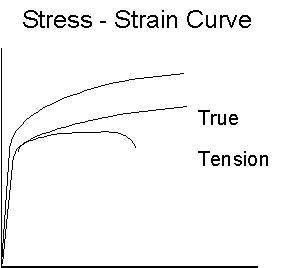
Stress-strain curve

For simplification, the stress-strain curve is divided into two regions. The steeply sloped region at very low strain values is known as the elastic region. In the elastic region, since strain is very low, when the material is unloaded and the forces removed, the material returns to its original shape. In Fig. AI.6., an object is deformed in uniaxial tension. The change in length is shown and the corresponding position on the stress-strain curve is shown. In this case, the deformation is completely elastic. After the tensile forces are removed, the material returns to the original shape.

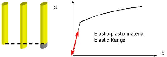
Diagram of elastic deformation

The second region of a stress-strain curve is known as the plastic region. This region comprises strains just above the elastic range and appear on the curve as the less steeply sloped region. In this region, the material does not recover any of the deformation that occurs. The only recovery that occurs is the accumulated elastic strain. In Fig. AI.7., a specimen under tension deforms first elastically and then plastically. The loading curve in Fig. AI.7. first follows the elastic loading curve and then follows the plastic curve. When the material is unloaded and the forces are removed from the specimen, the material follows the elastic curve down. When the material is completely unloaded, the deformation left over is the permanent deformation of the body.

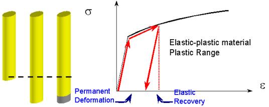
Diagram of plastic deformation

In DEFORM, the stress and strain used in the stress-strain curves are known as the effective stress and effective strain. The equations for these values are as seen below in Fig. AI.8.

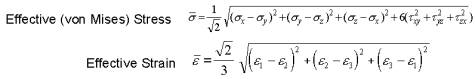
Equations for effective stress and strain

In DEFORM, the concept of flow stress is used. The idea of flow stress is important in case of incremental plasticity. As a material is deformed plastically, the amount of stress required to incur an incremental amount of deformation is given by the flow stress curve (which corresponds to the plastic region of the true stress-true strain curve). In Fig. AI.9., the concept is shown visually.

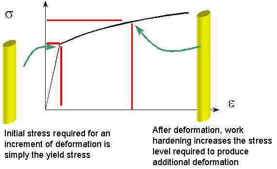
Introduction to flow stress concept

Flow stress is strongly dependent on several state variables, among these are accumulated strain, instantaneous strain rate and current temperature. As seen in Fig. AI.10., the flow stress curves can vary strongly with these state variables. So, it is important to account for these variables to accurately determine the behavior of the material.

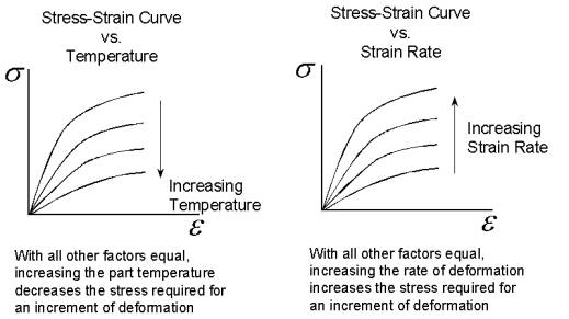
Variation of flow stress with strain rate and temperature

In the case where elastic deformation can be neglected, as in the case of bulk metal forming, the Levy-Mises flow rule can be used to relate the stress tensor to the strain rate tensor. This flow rule is shown in Fig. AI.11. The coefficient, l, is a function of state variables and the material. This relation allows one to express stress in terms of rate of deformation.

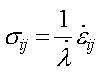
Levy-Mises flow rule

In calculating metal flow, the minimum work rate principle is a cornerstone for accurate calculation. This principle is defined below:

Minimum Work Rate Principle : The velocity distribution which predicts the lowest work rate is the best approximation of the actual velocity distribution.

This principle states that the material should always flow in the path of least resistance. This is shown in Fig. AI.12. where there are three different upset cases and the amount of friction between the workpiece and the tool determines the flow pattern of the material. In case of no friction, there is no resistance for the material from flowing straight out uniformly. In case of high friction, there is much resistance from flowing outward, so a barreling behavior is observed.

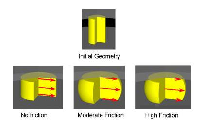
Minimum work rate principle

Note for each case, the actual velocity is the one which incurs the lowest work rate for the workpiece.

This minimum work rate principle can be expressed mathematically as the following functional form seen in Fig. AI.13. The top equation is simply a balance of the body forces (1st term) versus the surface tractions (2nd term). The manner in which this equation is solved for the velocities, is seen in the 2nd equation. The velocities are solved by solving for when the variation in the functional is stationary. Note that there is an extra term that maintains incompressibility in the solution. This is done by integrating the volumetric strain rate and multiplying by a large constant. Since the total solution should be zero, the solution will tend to maintain a low volumetric strain rate to keep this integral value low.

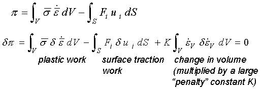
Functional equation for minimum work rate principle

In order to obtain a closed form solution for complex shapes, we need to resort to mathematical tricks such as FEM. The introductory theory for this is discussed in the following section.

Introduction to FEM theory

The principle of FEM theory is divide and conquer. First, one must divide the problem into small little subproblems that are easy to formulate and after the entire problem has been divided and formulated, they must all be carefully combined and then solved. The manner in which a problem is divided is through a process called meshing. In Fig. AI.14., an axisymmetric body is being upset between two flat dies. There is a grid that has been superimposed on the figure of the workpiece. This grid is the mesh that represents the body being deformed. Each rectangle represents a portion of material, in this case each rectangle corresponds to a ring, for which the equation in Fig. AI.13. can be easily solved. Each rectangle is called an element and the intersection of any grid lines is called a node. An element corresponds to a region of material and a node corresponds to a discrete point in space.

The solution for the equations in Fig. AI.13. are the velocity at each node, which are shown as vector arrows to the right side of Fig. AI.14. In additions to the bottom equation of Fig. AI.13., there are boundary conditions that should be specified in order to provide a unique solution to the problem. In this problem, the velocity of the top set of nodes is determined by the downward speed of the die as well as the friction model between the workpiece and the die. The boundary conditions on the left side of the die is specified as a centerline condition meaning that the nodes are not allowed to move either right or left. The bottom nodes also have a symmetry condition meaning that they are not allowed to move up or down. These three boundary conditions allow the mesh to behave as the actual part.

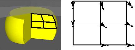
2D mesh of upset test

Note: This mesh is extremely coarse for the sake of clarity.

When the velocity at node points have been determined, their coordinates need to be updated. The manner in which we update the nodal coordinates is by integrating the velocity over the time step of the current step. In Fig. AI.15., the nodal positions are shown as updated from the previous stage. A simple principle of nodes are clear from this figure:

If the nodal velocities change direction or magnitude over very small time periods, a small time step size is required to correctly predict this behavior.

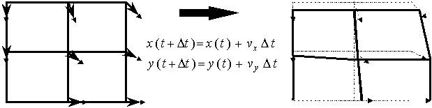
Updating nodal coordinates after a completed calculation

The problem that now must be addressed is how to solve the equation in Fig. AI.13. over a discrete set of points since the nodal values define the velocities only at discrete locations. The way in which to solve this problem is to define shape functions over the elements as a manner of providing a velocity field that satisfies the compatibility requirement (continuous over the entire body). Fig. AI.16. shows a general equation for a shape function whose purpose is to define the velocity profile over an element based on the nodal velocities. A one-dimensional case is shown in Fig. AI.16. as a simple linear function. The advantage of an equation of this form is that compatibility is maintained when the same nodes for any shared element edge, define the velocity over that edge.

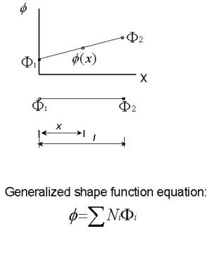
Description of a shape function

Fig. AI.17 also shows the case of a two-dimensional element.

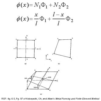
Description of shape function

After all the equations for the elements have been written out, they must be combined into a single set of simultaneous equations. This process is shown in Fig. AI.18. At the end, using a Newton-Raphson iteration method, the updated velocity can be solved for by solving a simultaneous set of equations. Once this velocity update is solved for, it is applied to the current velocity and velocity update is solved again.

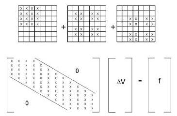
Construction of a stiffness matrix to solve for velocities

The general FEM solution process is given below:

1. Input Geometry & Processing Conditions.

2. Generate Initial Guess of Velocity Field single step.

3. Calculate Element Behavior Based on Velocity Field & other variables (strain, temp, etc).

4. Calculate Force boundary conditions based on Velocity Field.

5. Assemble and solve the matrix equation.

6. Calculate the error.

7. If error is too large, apply correction to velocity field and go to step 3. Otherwise, continue to step 8.

8. Update Geometry.

9. Calculate temperature change for this step.

10. Calculate new press velocity if necessary.

11. If stopping criteria has been reached, END. Otherwise, go to step 3 and repeat the process.

Modeling Material Behavior in FEM

Material Definition :

Flow stress in DEFORM is defined as a function of strain, strain rate and temperature.

In general DEFORM material data represents a single history. Separate data sets represent different histories,

• as received

• annealed

• spheroidized

• grain size

Finite Element Method Single Element Behavior:

Flow stress data gives force and energy required to deform the element. Equivalent calculations on other elements, and friction behavior give external forces. (See Fig. AI.19.)

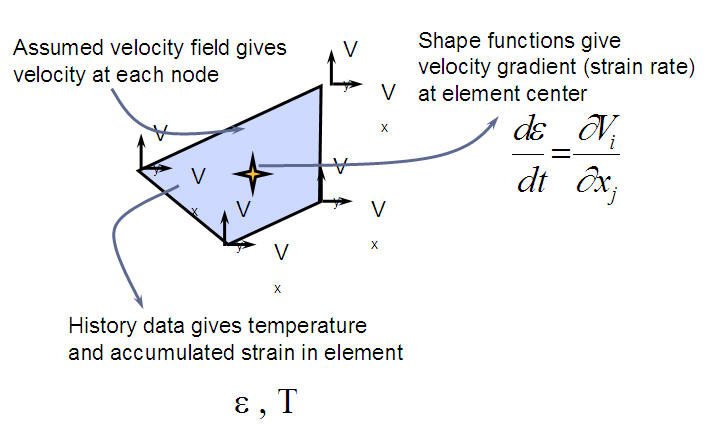
Single element behavior

This concludes short summary of the FEM process in metalforming. For more information on FEM theory, please consider reading the following list of references:

1. Kobayashi, S., Oh, S.I. and Altan T. Metalforming and the Finite-Element Method. Oxford University Press. 1989.

2. Przemieniecki, J.S. Theory of Matrix Structural Analysis. Dover Publications. 1968.

3. Zienkiewicz, O.C. and Taylor, R.L. The Finite Element Method. McGraw-Hill. 1989.