2D Machining Distortion Lab1

1.1. Creating a New problem

1.2. Adding operation

1.3. Object window

1.4. Workpiece

1.5. Setting up the fixtures

1.6. Defining the initial machining pass

1.7. Positionong

1.8. Scheduled Positioning

1.9. Contact

1.10. Simulation Preview

1.11. Simulation control

1.12. DB generation

1.13. Starting the Simulation

1.14. Post processing the results

Creating a New problem

On a Windows machine , go to the button select DEFORM-v1x.xxx (.xxx indicates version number E.g. v14.0.2) and select DEFORM GUI Main vxx.xx from the menu. The DEFORM GUI Main window will appear, as shown below Fig. 2DMDL1.1.

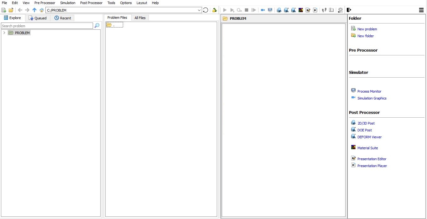
DEFORM GUI main window

Create a new problem either by selecting File New Problem or by clicking the New Problem icon. The Problem Setup window will appear as shown in Fig. 2DMDL1.2. Select “Integrated Manufacturing Process “ radio button and unit system as “English “ radio button in unit field. Define Problem Name as “2D_Machining_Distortion “ and make sure the “Show option dialog ” check box is turned on (if we do not turn on the “Show option dialog” check box, then we will not get the New Project dialog). Then click on button to open a new problem using the Deform Integrated Manufacturing Process.

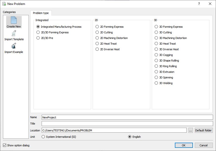
Problem type selection window

Multiple operation wizard will open, at this point user will be prompted to specify a project name (system will create a separate folder with this project name) and title for this session. In this session we use ‘2D_Machining_Distortion ’ as the project name ( see Fig. 2DMDL1.3.). Click on to continue to open the operation.

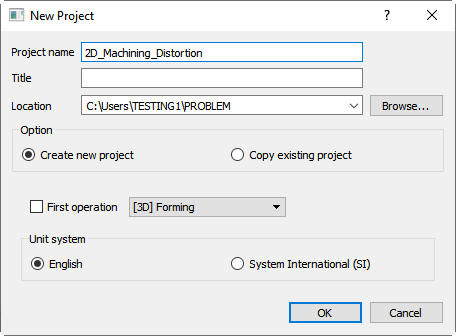
New project window

Adding operation

Multiple Operation wizard will open. Add 2D Machining Distortion operation from the Explorer Operations list. Operation can be add by clicking on 2D Machining Distortion operation button or user can also add by drag and drop into the Operation Editor (see Fig. 2DMDL1.4.).

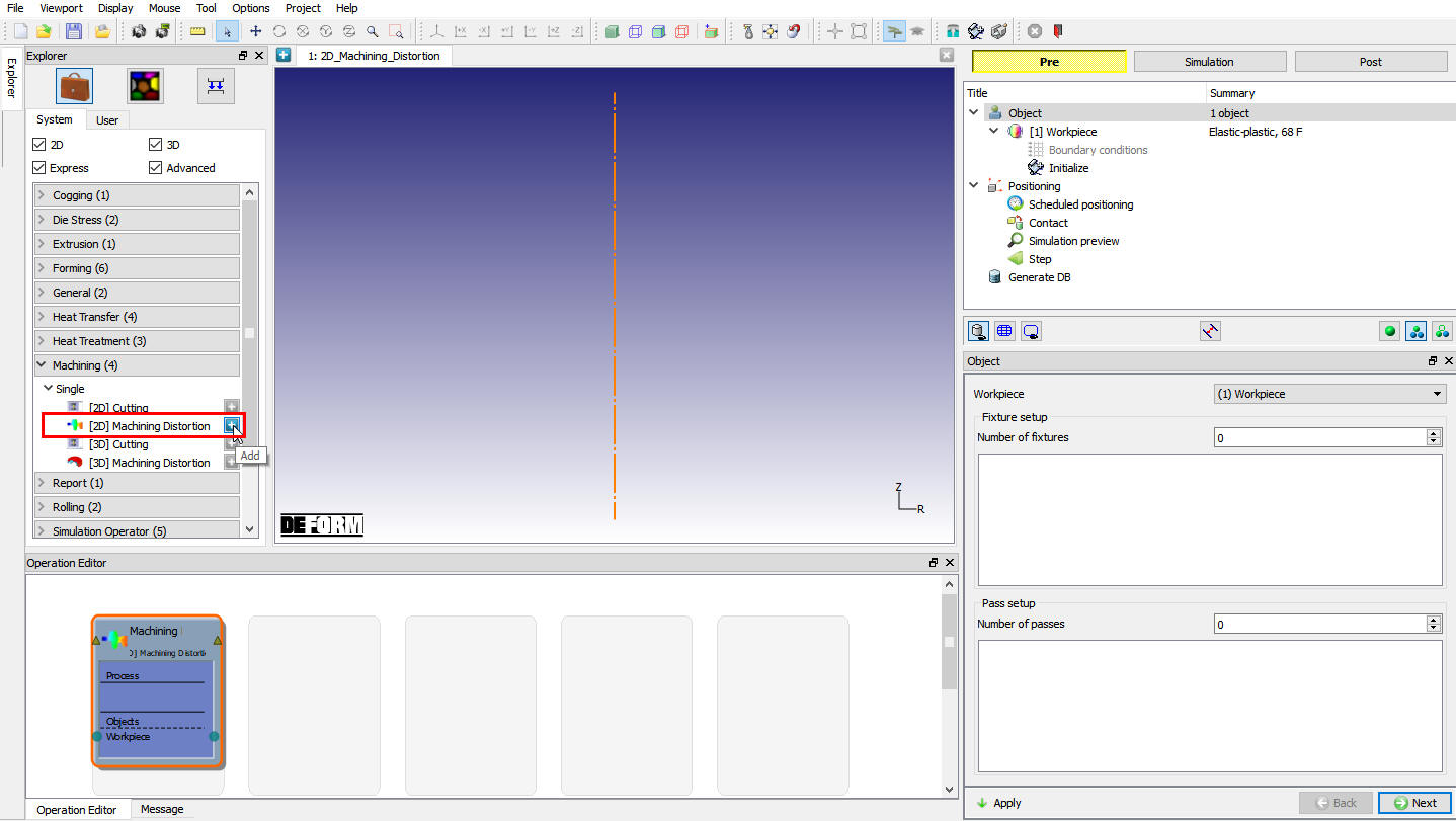
Adding 2D Machining Distortion operation

Object window

In the object window, for this lab along with workpiece 4 fixtures and 1 pass is required, so define the Number of fixtures as 4 and Numberof passes as 1 (see Fig. 2DMDL1.5.). Click on to add objects and click on .

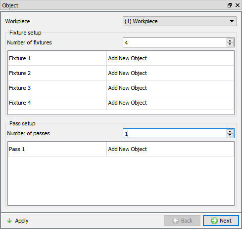
Object window

Workpiece

Inside this operation, load the object information by selecting option. User can browse for the database file. Load the file ‘CoolingModel.DB ’ from Deform Installation path *\2d\LABS\Machining_Distortion* and select the appropriate step number (last step for this lab) and object (this model has only one object) (see Fig. 2DMDL1.6.). For this lab two files are provided. One keyword file and one database file for a typical cooling simulation. The keyword file provided here was run to generate the database file. Once the object is loaded user can change the name of the object and select on ‘init displacement’ so that the distortion due to the material removal alone can be properly recorded. click on .

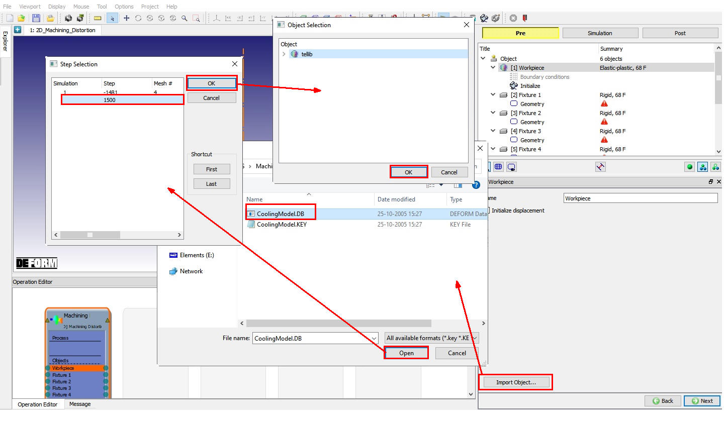
Workpiece Importing window

The object loaded comes with a set of deformation boundary conditions from the previous cooling simulation. User can verify these in the following Boundary conditions window ( Fig. 2DMDL1.7.) and click on to continue.

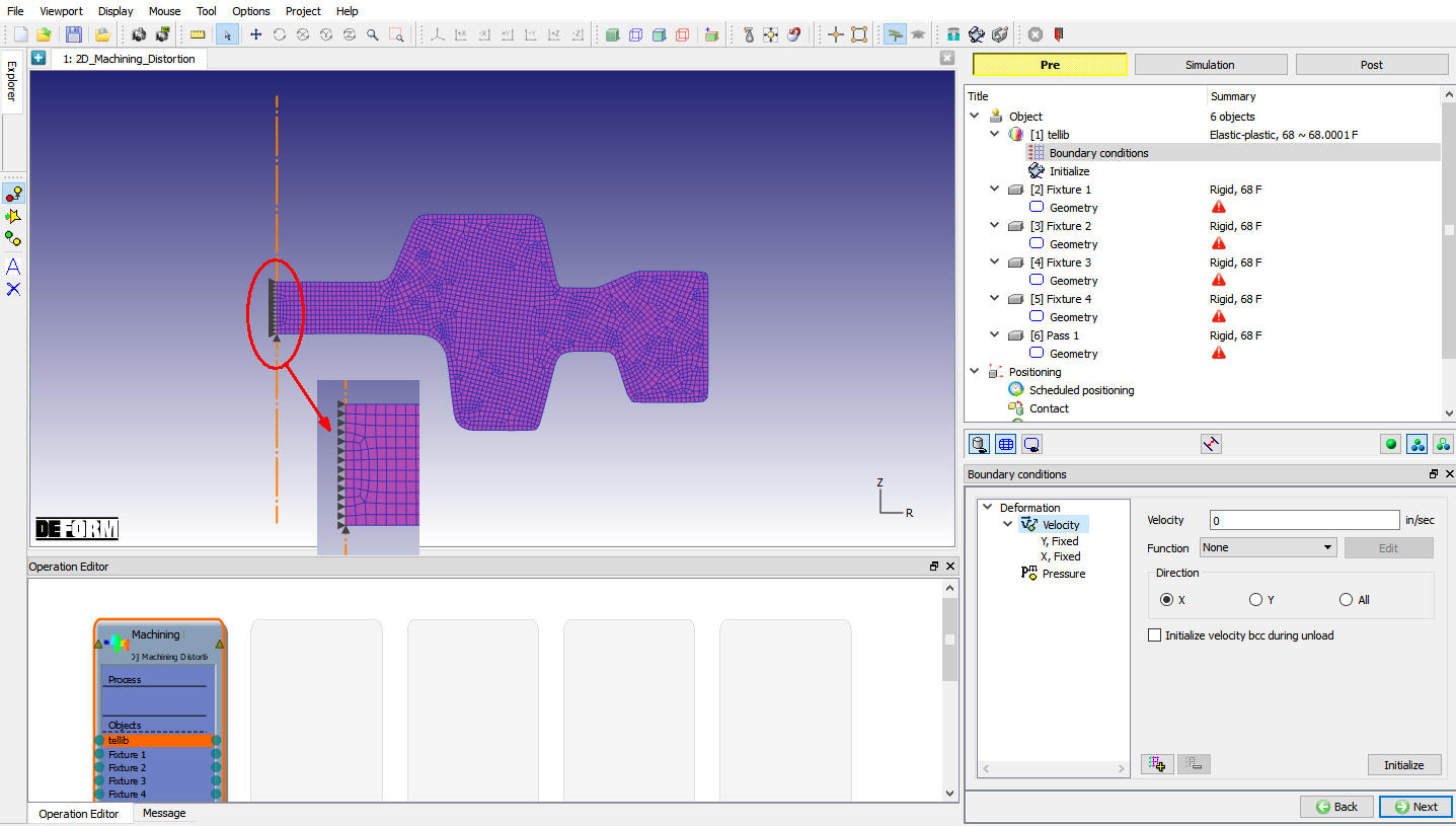
Boundary conditions window

In Initialize window, few state variables that are commonly used such as Temperature, strain, stress, damage, velocity, Displacement, etc.., are made available for initialization (see Fig. 2DMDL1.8.). Click on to continue.

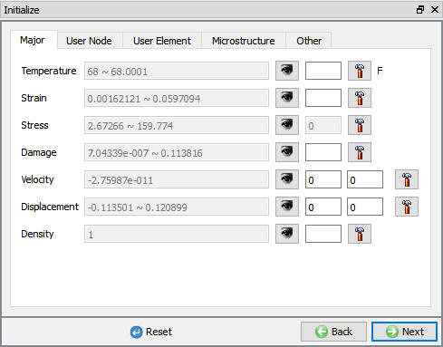
Initialize Window

Setting up the fixtures

Number of fixtures are added as four previously in Object window, This lab uses four fixtures. Two near the axis and two near the far end. They can be loaded (or defined) in any sequence. Once loaded, user can check the geometry and edit the same if needed.

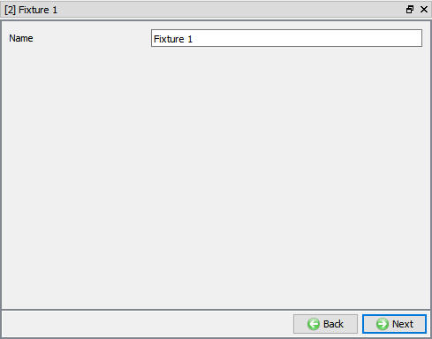
Fixture 1

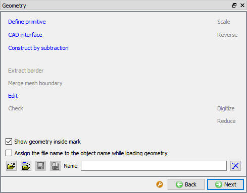
In the fixture 1 window, define the fixture name (if need different from the default one), and click on to load/define the fixture geometry. ( Fig. 2DMDL1.9.) Fixture geometry can be defined using the primitives, (which can also be edited interactively if needed) or load an existing geometry file ( see Fig. 2DMDL1.10.). For this lab, using the (Import Geometry from library) optionwe load the fixture 1 as bottom left one (lb_fixture.GEO) from Installation path \2d\LABS\Machining_Distortion folder .

Fixture 2

Similarly as Fixture 1, for Fixture 2 load upper left one (lu_fixture.GEO) from Installation path \2d\LABS\Machining_Distortion folder.

Fixture 3

Similarly as Fixture 1, for Fixture 3 load bottom one (rb_fixture.GEO) from Installation path \2d\LABS\Machining_Distortion folder.

Fixture 4

Similarly as Fixture 1, for Fixture 4 load right top one (ru_fixture.GEO) from Installation path \2d\LABS\Machining_Distortion folder.

Fixture 1 window

Geometry window

Defining the initial machining pass

From the model point of view, the machining pass information is also a geometry data, which when overlapping with the billet, decides the location and the extent of the material set for removal. Hence this is also a geometry data that can be defined/loaded in the same manner as the fixtures done in the last step. Using the (Import Geometry from library) option load the file ‘pass1.GEO ’ from Installation path \2d\LABS\Machining_Distortion folder as shown in Fig. 2DMDL1.12. User can check this geometry.

Pass window

Geometry window

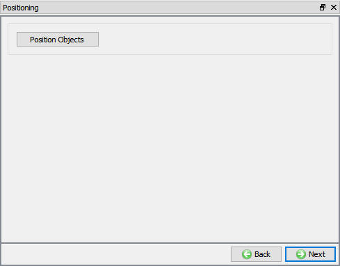
Positioning

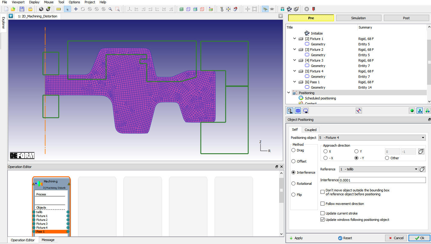
In this operation we position the fixtures with respect to the billet, so that they represent the proper constraints on the billet as the machining sequence is carried out. Select option to enter the ‘Object Positioning’ dialog. Here select the ‘Interference ’ mode of positioning. From the object list select ‘Billet’ as the reference object, and sequentially select fixtures 1 to 4 for positioning. ( Fig. 2DMDL1.13.) For each pair correct approach direction should be selected for positioning. Approach direction for bottom fixtures should be ‘Y’ and top fixtures ‘-Y’. User can use the default interference value and click on to carry out the positioning for each fixture (See Fig. 2DMDL1.14.).

Controls window

Position objects window

Scheduled Positioning

Schedule positioning allows the user to define the positioning for objects in MO setup for successive operations for which DB is not generated so that the objects are positioned before generation of DB while running simulation in batch mode. For this lab we are not using this scheduled positioning.

Contact

In this stage we define ‘4’ pairs of master-slave objects. First enter the Contact and in the Contact dialog, click on (Add relationship) four times to indicate four pairs of objects. For each pair sequentially select one fixture as master and billet as slave. For this lab we do not define any friction conditions. (user can enter (Edit) option to define friction conditions if needed) or user can directly click on the to add the all default relations. Click on to generate the contact conditions ( Fig. 2DMDL1.15.). At this stage contact nodes will be highlighted in the display area. Click on to continue.

Contact window

Simulation Preview

Simulation Preview provides an overview of the operation to be executed based on the process definition and pass. In Simulation preview window (see Fig. 2DMDL1.16.), by clicking the (Play Preview Forward) button animation would be played and shows the object that as removed after the pass (see Fig. 2DMDL1.17.). Click on to continue.

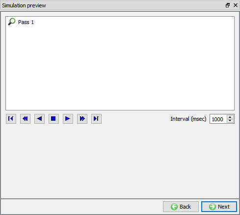
Simulation preview window

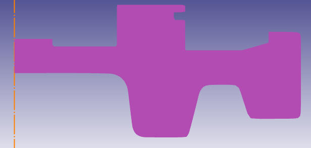
Preview of the setup

Simulation control

Last step of the model data generation is to set up the simulation controls where we define starting step as ‘-1’, number of steps as ‘2’ saving every step, and ‘1 sec’ time per step. Click on to enter the database generation page.

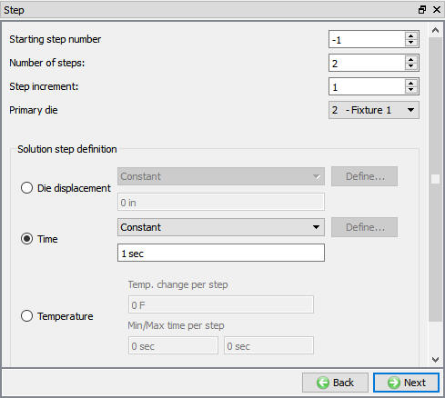
Simulation control Simulation Mode options

DB generation

In Generate DB page. Click on the button to generate the database. Observe the message in Message tab informing database generation status as shown in Fig. 2DMDL1.19. When the program is done writing the database, switch to tab to run simulation.

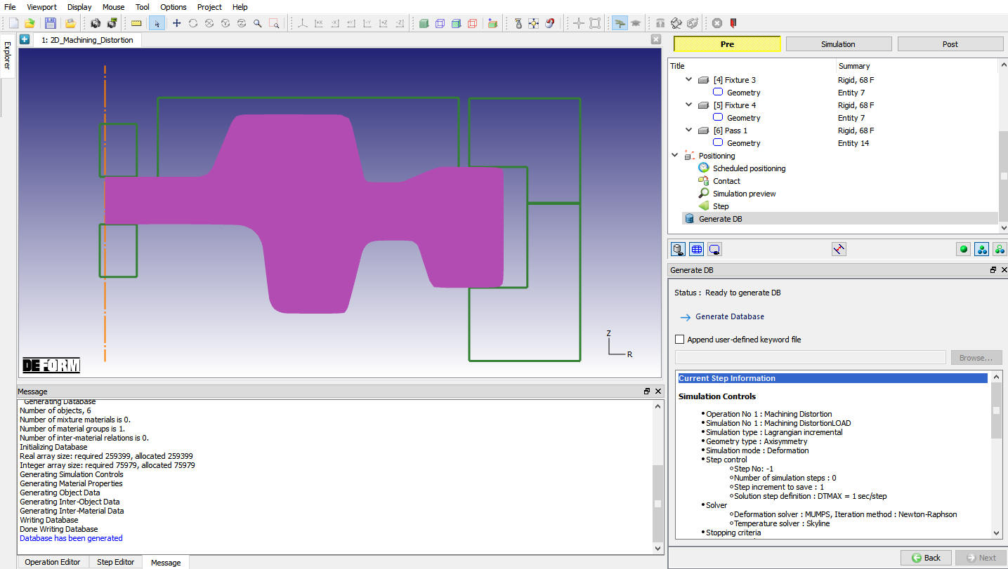
Generate Database window

Starting the Simulation

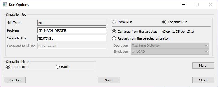
Click on the action label under the simulation tab, Run Options dialog will open as shown in Fig. 2DMDL1.20.. Use the default Continue Run option to select “Continue from the last step ” option and then select the Simulation mode as Interactive and click on button to run the simulation.

When the simulation is finished we can observe that the following message is added to the end of the Message file:

**Message***

Simulation is completed and stopped at the user specified time step.

Simulation tab to submit simulation

Post processing the results

After the simulation is complete, user can enter to see the model results. Typical sequence is to first select the step number, and then the state variables to be displayed. Some important state variables can be selected directly from post and the rest can be access through table (by selecting). Fig. 2DMDL1.21. indicates the effective stress distribution after the machining pass and Fig. 2DMDL1.22. indicates maximum principal stress distribution after machining pass.

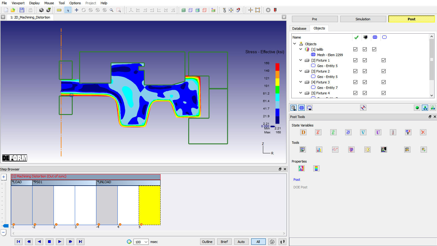
Effective stress distribution and distorted billet after the machining pass

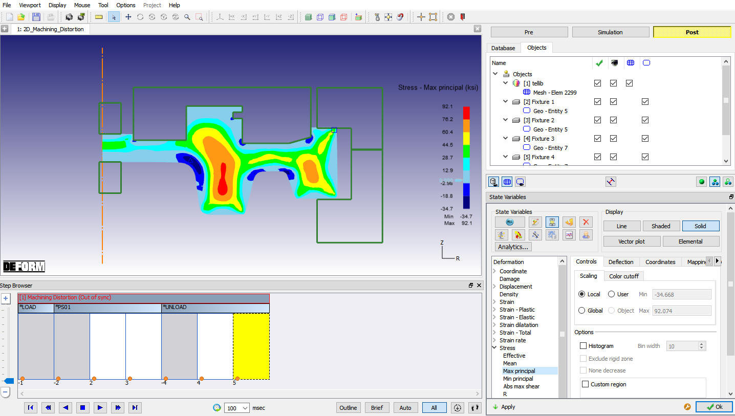
Max. Principal stress distribution and distorted billet after the machining pass